Deep Learning for traffic prediction [project with source code]

• Introduction
• Data
• Preprocessing the data
• The Model

Introduction

This article at OpenGenus explores the development of a Deep Learning (DL) traffic predictor using a comprehensive dataset. The objective is to construct a model capable of forecasting traffic flow over a twelve-hour span in a major U.S. metropolitan area. The data encompasses temporal, spatial, and directional attributes, allowing for intricate modeling of interactions across a network of roadways.

All the code used for the graphs and models can be found in the following notebook Kaggle: Your Home for Data Science

Data

In this competition, you'll forecast twelve-hours of traffic flow in a major U.S. metropolitan area. Time, space, and directional features give you the chance to model interactions across a network of roadways.

This dataset was derived from the Chicago Traffic Tracker - Historical Congestion Estimates dataset.

comprising measurements of traffic congestion across 65 roadways from April through September of 1991.
- row_id - a unique identifier for this instance
- time - the 20-minute period in which each measurement was taken
- x - the east-west midpoint coordinate of the roadway
- y - the north-south midpoint coordinate of the roadway
- direction - the direction of travel of the roadway. EB indicates "eastbound" travel, for example, while SW indicates a "southwest" direction of travel.
- congestion - congestion levels for the roadway during each hour; this is the target variable. The congestion measurements have been normalized to the range 0 to 100.

To get a deeper understanding of the data, the exploratory data analysis by Kelli Belcher is an excellent resource, but too avoid spending this whole article diving into the EDA and the data to instead focus on the model building, its enough to know some basics, starting with understanding the geography of the roads we're trying to predict the congestion for:

Road Geography

We know that every unique x value represents a certain roads east-west coordinate while the y-value represents the north south value. So to generate a list of the unique roads we can simply use the following code:

# Unique roads
roadways = train[['x', 'y']].drop_duplicates()
print(roadways)

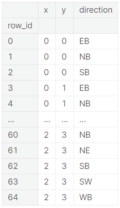
On top of this we also have the directions variable, and if we combine all of the unique roads with the unique directions we get all the possible congestion points.

# Unique roadways with direction
road_dir = train[['x', 'y', 'direction']].drop_duplicates()
print(road_dir)

As we can see in the list, there are 64 unique combinations of roads and directions, these can be plotted in the following way to get a better understanding of what the road network looks like (code taken from AMBROSMs excellent notebook)

dir_dict = {'EB': (1, 0), 'NB': (0, 1), 'SB': (0, -1), 'WB': (-1, 0), 'NE': (1, 1), 'SE': (1, -1), 'NW': (-1, 1), 'SW': (-1, -1)}

plt.figure(figsize=(8, 8))
plt.scatter(roadways.x, roadways.y)
plt.gca().set_aspect('equal')
for _, x, y, d in road_dir.itertuples():
    dx, dy = dir_dict[d]
    dx, dy = dx/4, dy/4
    plt.plot([x, x+dx], [y, y+dy], color='#ffd700')
plt.gca().xaxis.set_major_locator(MaxNLocator(integer=True)) # only integer labels
plt.gca().yaxis.set_major_locator(MaxNLocator(integer=True)) # only integer labels
plt.xlabel('x')
plt.ylabel('y')
plt.show()

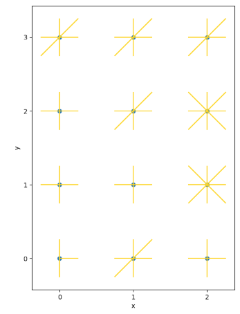
With this understanding of the geography of the roads, we can make some remarks:

• Congestion at specific spatial points and directions should be correlated to the congestion at nearby points in that direction. (this means that for example congestion at (0,0, northbound) should be correlated with later congestion at (0 , 1)).
• Although the y coordinate in the diagram grows from bottom to top (south to north), we can't take this for granted. Maybe it should grow from top to bottom.

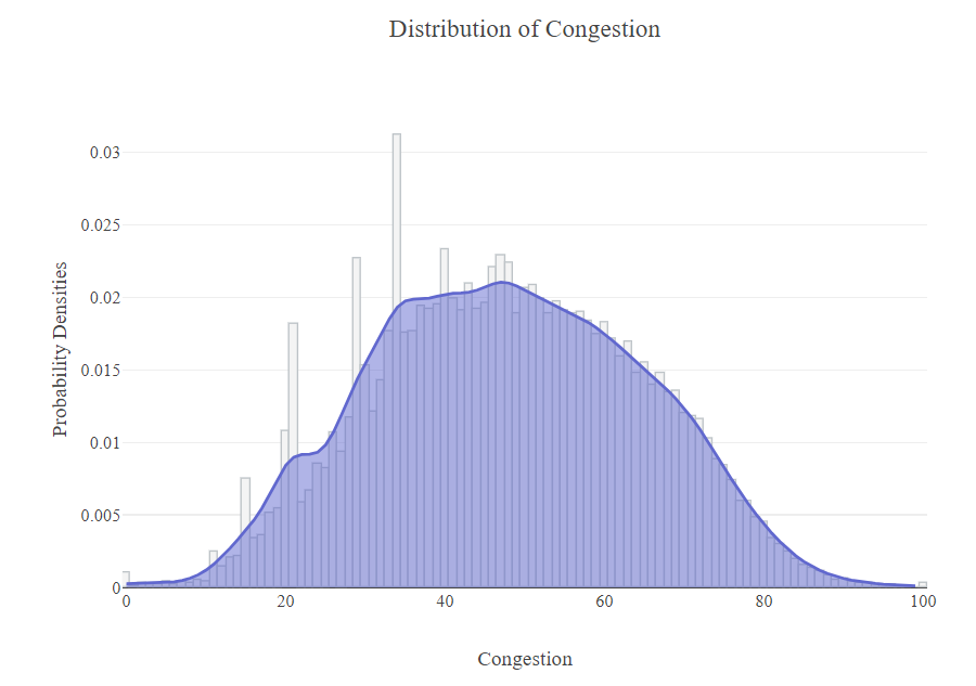
The Congestion Variable

At a first look of the distribution of the Congestion variable we can see that its approximately normally distributed, but some variable (15, 20, 21, 29, 34) are overrepresented.

if we want to look at the congestion with relation to the unique roads and directions the following code generates the necessary plots

for direction in train.direction.unique():
    temp = train[(train.x == 2) & (train.y == 1) & (train.direction == direction)]
    plt.subplots(1, 2, figsize=(18, 4))
    plt.subplot(1, 2, 1)
    vc = temp.congestion.value_counts().sort_index()
    plt.bar(vc.index, vc, width=1,
            color=['r' if con in [15, 20, 21, 29, 34] else '#ffd700' for con in vc.index])
    plt.ylabel('Count')
    plt.xlabel('Congestion')
    plt.title(f"(x = {2}) & (y = {1}) & (direction = {direction})")
    plt.subplot(1, 2, 2)
    plt.scatter(temp.time, temp.congestion, s=1, color=['r' if con in [15, 20, 21, 29, 34] else '#ffd700' for con in temp.congestion])
    plt.title(f"(x = {2}) & (y = {1}) & (direction = {direction})")
    plt.ylabel('Congestion')
    plt.show()

Below are some of the generated plots, since there will be a lot of plots in total I chose to just include a sample to show the variability within the distributions for some different roads and directions.

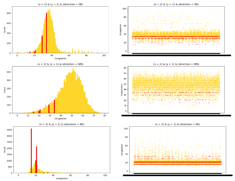
Given the variability within the dataset, its clear that linear regression would not be suitable for modeling. Decision trees or deep learning would be a more appropriate choice to handle and capture the complexities of the data.

Preprocessing the data

When it comes to preparing the data for the model some of the variables need to be edited so they can be better used. Since a lot of models only accept integer values a good place to start is with the none integer values: Time and Direction.

Encoding Direction

One of the key data preprocessing steps involved dealing with the categorical variable Direction. To make this categorical information usable for machine learning algorithms, I applied one-hot encoding. By doing so, I expanded the Direction column into multiple binary columns, each representing a unique direction category. This transformation effectively converted categorical data into a format that the model can comprehend.

Extracting Time Features

The "Time" variable is another pivotal factor that can significantly impact the model's performance. However, raw timestamps aren't directly interpretable by machine learning algorithms. Therefore, I dissected the "Time" information into several meaningful features that can effectively capture temporal patterns and trends.

The following time-related features were extracted from the "Time" variable and added to the dataset:

• Weekday: This feature captures the day of the week, with Monday represented as 0 and Sunday as 6.
• Month: The numerical representation of the month.
• Daytime: The time of day converted into minutes since midnight.
• Day of Year: The day's position in the year, facilitating the modeling of annual trends.

# Create a new DataFrame with one-hot encoded direction columns
direction_encoded = pd.get_dummies(train_df['direction'], prefix='direction')
train_df = pd.concat([train_df, direction_encoded], axis=1)

# extract the time fetures from '1991-06-03 14:40:00' 
#into integer for day month week weekday etc 
train_df['time'] = pd.to_datetime(train_df['time'])
train_df['weekday'] = train_df.time.dt.weekday  # Monday is 0 and Sunday is 6
train_df['month'] = train_df['time'].dt.month
train_df['daytime'] = train_df.time.dt.hour * 60 + train_df.time.dt.minute
train_df['dayofyear'] = train_df.time.dt.dayofyear # to model the trend

# Exclude 'row_id','time', direction and the target variable columns
columns_to_exclude = ['row_id', 'time','direction','congestion']
X = train_df_1.drop(columns=columns_to_exclude)

# Standardize the values using StandardScaler
scaler = StandardScaler()
X_standardized = scaler.fit_transform(X)

# Create a new DataFrame with standardized values and original columns
X_standardized_df = pd.DataFrame(X_standardized, columns=X.columns)
# Separate the target variable
y = train_df_1['congestion']

# Split the data into training and validation sets
X_train, X_val, y_train, y_val = train_test_split(X_standardized_df, y, test_size=0.2, random_state=42)

The Model

I choose to apply a rather simple model with only tree layers. This was done to minimize the computational resources needed to train it. Below follows a deeper explanation about what is involved in the model.

# Create a deep learning model
model = Sequential()
model.add(Dense(64, activation='relu', input_dim=X_train.shape[1]))
model.add(Dense(32, activation='relu'))
model.add(Dense(1, activation='linear'))

# Compile the model
model.compile(optimizer='adam', loss='mean_squared_error')

# Set up early stopping
early_stopping = EarlyStopping(patience=10, restore_best_weights=True)

The model architecture is built using the Keras framework, employing the Sequential model type. This type of model allows for the construction of a linear stack of layers, facilitating the flow of information from input to output.

1. Input Layer (Dense Layer with ReLU Activation): The first layer of the model is a dense layer with 64 units. This layer acts as the initial point of entry for the preprocessed data. The activation function used here is ReLU, which introduces non-linearity into the model. The number of units in this layer, 64, is a hyperparameter that can be adjusted based on the complexity of the problem and the dataset.
2. Hidden Layer (Dense Layer with ReLU Activation): The subsequent layer consists of 32 units and also employs the ReLU activation function. This hidden layer is responsible for further abstracting and learning complex patterns within the data.
3. Output Layer (Dense Layer with Linear Activation): The final layer of the model has a single unit, designed for regression tasks where the goal is to predict a continuous value. The activation function used here is linear, which directly provides the model's prediction as an output.

Model Compilation

After defining the model architecture, the next step is to configure the model for training by specifying the optimizer and loss function.

• Optimizer (Adam): The Adam optimizer, a variant of stochastic gradient descent, is chosen for its adaptive learning rate and efficient optimization capabilities. It dynamically adjusts the learning rate during training, leading to quicker convergence.
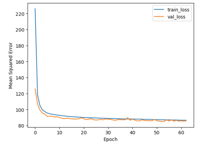
• Loss Function (Mean Squared Error): The mean squared error (MSE) is utilized as the loss function. In regression tasks like this one, where the goal is to predict continuous values, MSE computes the average of the squared differences between the predicted and actual values. Minimizing this loss function encourages the model to make predictions that are as close as possible to the ground truth.

Early Stopping

To prevent overfitting and ensure optimal generalization, an early stopping mechanism is employed. This technique monitors the validation loss during training and halts the training process if the loss does not improve for a defined number of epochs (patience). This strategy helps in selecting a model that performs well on unseen data and avoids unnecessary overfitting.

Training & Results

For the training of the model I decided to limit the data used to 20% of the data available in the data set, this was done since the dataset is truly massive and my computer had a hard time dealing with it.
Using this subset of the data also seemed to be enough to train the model and get decent predictions.

Here are the predictions vs the actual values for the validation data for 2 different roads:

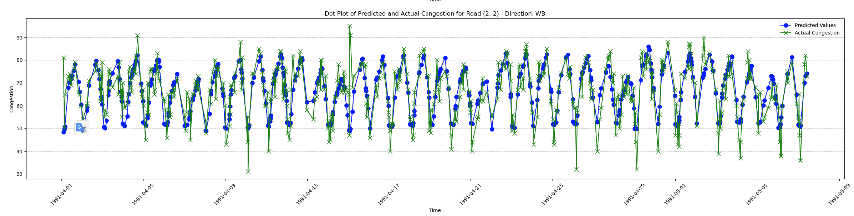
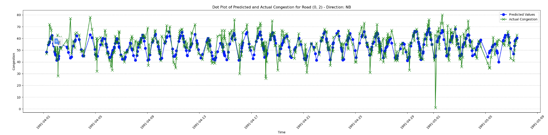
Here we can see that that although the model sometimes has a hard time predicting rapid changes in congestion, it performs generally well.