Gradient clipping in DL

Gradient clipping is a technique commonly used in deep / machine learning, particularly in the training of deep neural networks, to address the issue of exploding gradients.

Exploding gradients occur when the gradients of the loss function with respect to the model's parameters become very large during training. This can lead to numerical instability and make it challenging for the model to converge.

Master Deep Learning with this checklist. This is a free 13 months course.

Table of contents :

• The Problem: Exploding Gradients
• The Solution: Gradient Clipping
• Gradient Clipping in Keras
• Regression Predictive Modeling Problem
• MLP With Gradient Value Clipping
• Hyperparameter Tuning
• Benefits of Gradient Clipping

The Problem: Exploding Gradients

When training neural networks using gradient-based optimization methods (e.g., stochastic gradient descent, Adam), the goal is to update the model's parameters in a way that minimizes a certain loss function. This is achieved by computing gradients of the loss with respect to the model's parameters and then adjusting the parameters in the opposite direction of the gradient.

However, in deep neural networks with many layers, the gradients can become very large during backpropagation. This phenomenon is known as "exploding gradients." When gradients are extremely large, they can lead to several problems:

• Numerical instability : Large gradients can result in numerical instability during the optimization process, causing weight updates to be extremely large or small, which disrupts convergence.
• Divergence : The optimization process may diverge, causing the loss to increase instead of decrease.
• Difficulty in convergence : The network may take a very long time to converge, or it may fail to converge at all.

The Solution: Gradient Clipping

Gradient clipping is a technique used to address the issue of exploding gradients by imposing an upper bound (a threshold) on the gradient values during training. Here's how it works in more detail:

• Compute Gradients :
  During the backward pass (backpropagation) of training, gradients are computed for each parameter in the neural network with respect to the loss function. These gradients indicate the direction and magnitude of parameter updates needed to minimize the loss.

• Calculate Gradient Norm :
  Calculate the norm (magnitude) of the gradients. The most commonly used norm is the L2 norm, which is calculated as the square root of the sum of the squares of individual gradient values.

• Clip the Gradients :
  If the gradient norm exceeds a predefined threshold (e.g., a hyperparameter you specify), gradient clipping comes into play. The gradients are rescaled or clipped to ensure that their norm does not surpass this threshold. There are two common approaches:

  • Fixed Threshold Clipping: All gradients are scaled down uniformly such that their overall magnitude doesn't exceed the threshold. This is done by dividing all gradients by the gradient norm if it's larger than the threshold.
    clipped_gradient = gradient * (threshold / gradient_norm)
  • Adaptive Threshold Clipping: Each gradient is scaled individually based on its own magnitude. This avoids overly aggressive clipping of gradients and is especially useful when gradients vary widely across parameters.
    clipped_gradient = gradient * (threshold / gradient_norm) if gradient_norm > threshold else gradient
  • Update Model Parameters: Finally, the clipped gradients are used to update the model parameters (e.g., weights and biases) via the chosen optimization algorithm (e.g., gradient descent, Adam). These clipped gradients ensure that the parameter updates are controlled and do not lead to numerical instability.

Gradient Clipping in Keras

Keras, which is a tool for building and training neural networks, has a feature called "gradient clipping." This feature helps make training neural networks more stable.

Imagine you're teaching a computer program to learn something, and you're using a special method to help it learn better. Gradient clipping is like making sure the program doesn't learn too quickly, which can cause problems. Instead, you want it to learn at a reasonable pace.

There are two ways gradient clipping works:

1. Gradient Norm Scaling: This is like checking how fast the program is learning. If it's learning too fast (more than we want), we slow it down a bit. We do this by making sure the speed of learning doesn't go above a certain limit. It's like saying, "You can't go faster than 1 mile per hour." If the program tries to go faster, we make it slow down.

   Gradient norm scaling involves changing the derivatives of the loss function to have a given vector norm when the L2 vector norm (sum of the squared values) of the gradient vector exceeds a threshold value.

   For example, we could specify a norm of 1.0, meaning that if the vector norm for a gradient exceeds 1.0, then the values in the vector will be rescaled so that the norm of the vector equals 1.0.
   This can be used in Keras by specifying the “clipnorm” argument on the optimizer; for example:

opt = SGD(lr=0.01, momentum=0.9, clipnorm=1.0) 

3. Gradient Value Clipping: This is like saying, "You can't learn too much in one go." If the program tries to learn too much at once, we limit how much it can learn in a single step. This helps keep things under control.
   Gradient value clipping involves clipping the derivatives of the loss function to have a given value if a gradient value is less than a negative threshold or more than the positive threshold.
   For example, we could specify a norm of 0.5, meaning that if a gradient value was less than -0.5, it is set to -0.5 and if it is more than 0.5, then it will be set to 0.5.

This can be used in Keras by specifying the “clipvalue” argument on the optimizer, for example:

opt = SGD(lr=0.01, momentum=0.9, clipvalue=0.5) 

Regression Predictive Modeling Problem

A regression predictive modeling problem involves predicting a real-valued quantity.

We can use a standard regression problem generator provided by the scikit-learn library in the make_regression() function. This function will generate examples from a simple regression problem with a given number of input variables, statistical noise, and other properties.

We will use this function to define a problem that has 20 input features; 10 of the features will be meaningful and 10 will not be relevant. A total of 1,000 examples will be randomly generated.

# generate regression dataset
X, y = make_regression(n_samples=1000, n_features=20, noise=0.1, random_state=1) 

Each input variable has a Gaussian distribution, as does the target variable.

We can create plots of the target variable showing both the distribution and spread. The complete example is listed below.

# regression predictive modeling problem
from sklearn.datasets import make_regression
from matplotlib import pyplot
# generate regression dataset
X, y = make_regression(n_samples=1000, n_features=20, noise=0.1, random_state=1)
# histogram of target variable
pyplot.subplot(121)
pyplot.hist(y)
# boxplot of target variable
pyplot.subplot(122)
pyplot.boxplot(y)
pyplot.show() 

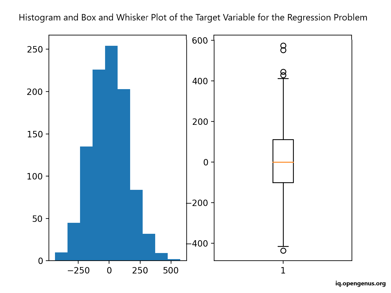
Running the example creates a figure with two plots showing a histogram and a box and whisker plot of the target variable.

The histogram shows the Gaussian distribution of the target variable. The box and whisker plot shows that the range of samples varies between about -400 to 400 with a mean of about 0.0.

MLP With Gradient Value Clipping

We can update the training of the MLP to use gradient clipping by adding the “clipvalue” argument to the optimization algorithm configuration. For example, the code below clips the gradient to the range [-5 to 5].

# compile model
opt = SGD(lr=0.01, momentum=0.9, clipvalue=5.0)
model.compile(loss='mean_squared_error', optimizer=opt)

The complete example of training the MLP with gradient clipping is listed below.

# mlp with unscaled data for the regression problem with gradient clipping
from sklearn.datasets import make_regression
from keras.layers import Dense
from keras.models import Sequential
from keras.optimizers import SGD
from matplotlib import pyplot
# generate regression dataset
X, y = make_regression(n_samples=1000, n_features=20, noise=0.1, random_state=1)
# split into train and test
n_train = 500
trainX, testX = X[:n_train, :], X[n_train:, :]
trainy, testy = y[:n_train], y[n_train:]
# define model
model = Sequential()
model.add(Dense(25, input_dim=20, activation='relu', kernel_initializer='he_uniform'))
model.add(Dense(1, activation='linear'))
# compile model
opt = SGD(lr=0.01, momentum=0.9, clipvalue=5.0)
model.compile(loss='mean_squared_error', optimizer=opt)
# fit model
history = model.fit(trainX, trainy, validation_data=(testX, testy), epochs=100, verbose=0)
# evaluate the model
train_mse = model.evaluate(trainX, trainy, verbose=0)
test_mse = model.evaluate(testX, testy, verbose=0)
print('Train: %.3f, Test: %.3f' % (train_mse, test_mse))
# plot loss during training
pyplot.title('Mean Squared Error')
pyplot.plot(history.history['loss'], label='train')
pyplot.plot(history.history['val_loss'], label='test')
pyplot.legend()
pyplot.show()

Running this example fits the model and evaluates it on the train and test sets, printing the mean squared error.

A line plot is also created showing the means squared error loss on the train and test datasets over training epochs.

The plot shows that the model learns the problem fast, achieving a sub-100 MSE loss within just a few training epochs.

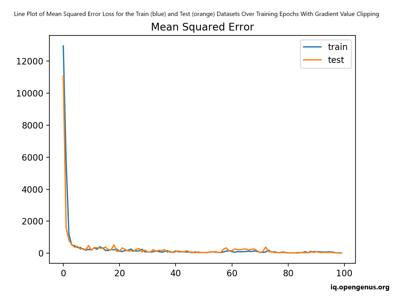
A clipped range of [-5, 5] was chosen arbitrarily; you can experiment with different sized ranges and compare performance of the speed of learning and final model performance.

Hyperparameter Tuning:

Choosing an appropriate threshold value is essential for effective gradient clipping. A threshold that is too small might prevent the model from learning, while a threshold that is too large might not effectively control exploding gradients. The threshold is typically considered a hyperparameter and may require experimentation to find the optimal value for your specific model and dataset.

Benefits of Gradient Clipping:

• Stability: Gradient clipping promotes stability during training, preventing extreme weight updates.
• Convergence: It helps the model converge faster and more reliably.
• Robustness: It makes it possible to train deep networks that might otherwise be challenging to optimize.