In this article at OpenGenus, we'll be diving into the world of deep learning and exploring some key terms / topics that you should be familiar with. Whether you're just starting out in the field or looking to expand your knowledge, understanding these concepts will be essential for your success in deep learning. So let's get started!

• Introduction
• Deep Learning
• Perceptron
• Multilayer Perceptron
• Backpropagation
• Gradient Descent
• Gradient Ascent
• Activation Function
• Loss Function
• Convolution
• MatMul
• Overfitting
  • Dropout
  • Early Stopping
• Convolutional Neural Networks(CNNs)
  • Pooling
  • Flatten
• Recurrent Neural Networks(RNNs)
  • LSTM
• Autoencoder
• Transfer Learning
• Generative Adversarial Networks(GANs)
• Artificial Neural Networks(ANNs)
• Hyperparameter
• Learning Rate
• Batch Normalization
• Quantization
• Inference
• Softmax
• Natural Language Processing(NLP)
  • NLP
  • Tokenization
  • Word Embedding
• Supervised Learning
  • Supervised Learning
  • Training Dataset
  • Validation Dataset
  • Testing Dataset
• Unsupervised Learning
• Reinforcement Learning
• Conclusion

Introduction

Deep learning is a rapidly growing field that is revolutionizing industries from healthcare to finance to self-driving cars. As artificial intelligence (AI) becomes more prevalent in our lives, it is important to have a basic understanding of the key terms and concepts that are used in deep learning.

This blog post aims to provide an overview of some of the most commonly used key terms in deep learning. From neural networks to convolutional neural networks, backpropagation to softmax, we will cover the most important concepts that you need to know to get started in deep learning.

Whether you are an aspiring data scientist or a seasoned machine learning professional, understanding these key terms is essential for developing and training accurate deep learning models. So, let's dive in and explore the world of deep learning!

Deep Learning

Deep learning is a subset of machine learning that involves training artificial neural networks with multiple hidden layers. It has rapidly become one of the most powerful techniques in the field of AI, enabling the development of sophisticated models that can solve complex problems such as image and speech recognition, natural language processing, and autonomous driving.

The key difference between deep learning and shallow learning is the number of layers in the neural network. In shallow learning, there are only one or two hidden layers between the input and output layers. This limits the ability of the model to learn complex patterns in the data. In contrast, deep learning models can have dozens or even hundreds of layers, allowing them to learn very complex patterns and relationships.

One of the main advantages of deep learning is its ability to automatically learn features from raw data, eliminating the need for manual feature engineering. This greatly reduces the amount of domain expertise required to build accurate models and allows deep learning to be applied to a wide range of domains.

However, deep learning also poses several challenges. One of the main challenges is the need for large amounts of training data. Deep learning models have a vast number of parameters and require a lot of data to learn accurate representations of the input. Another challenge is the difficulty in interpreting the models. Deep learning models are often described as "black boxes," meaning that it can be difficult to understand how they arrive at their predictions.

In conclusion, Deep Learning is a powerful subset of machine learning that enables the development of sophisticated models capable of solving complex problems. Its ability to learn features automatically from raw data is a significant advantage, but the need for large amounts of training data and the difficulty in interpreting models remain challenges.

Perceptron

Perceptron is a type of artificial neural network that is composed of a single layer of input nodes and output nodes, and sometimes a bias node. The input layer receives the inputs, which are then weighted and summed up, and passed through an activation function to produce the output. The activation function is usually a simple threshold function that decides whether the output should be 0 or 1, based on the weighted sum of inputs.

The perceptron was one of the earliest neural network architectures, and was first proposed in the 1950s by Frank Rosenblatt. It was originally designed as a binary classifier, and could be trained using a simple algorithm called the perceptron learning rule. This algorithm adjusts the weights of the inputs based on the difference between the actual output and the desired output.

Despite its simplicity, the perceptron has been shown to be capable of solving a wide range of classification problems. However, it has a limitation in that it can only solve linearly separable problems. That is, it can only classify data that can be separated by a single straight line. This limitation led to the development of more complex neural network architectures, such as multi-layer perceptrons, that are capable of solving non-linearly separable problems.

Multilayer Perceptron(MLP)

A Multilayer Perceptron (MLP) is a type of artificial neural network that is commonly used for classification and regression tasks. It is a feedforward network, which means that the information flows in one direction, from the input layer to the output layer, without any feedback loops. The MLP consists of one or more hidden layers of neurons, which are sandwiched between the input and output layers.

The input layer of the MLP receives the input data, which is then processed by the hidden layers through a series of linear and non-linear transformations. Each neuron in the hidden layers receives input from the neurons in the previous layer, applies an activation function to the weighted sum of its inputs, and passes the output to the next layer. The output layer of the MLP produces the final result, which could be a classification label or a numerical value.

During training, the MLP adjusts its weights and biases using an optimization algorithm such as gradient descent in order to minimize a loss function that measures the difference between the predicted output and the actual output. The backpropagation algorithm is used to calculate the gradients of the loss function with respect to the weights and biases, and these gradients are used to update the network parameters.

MLPs have been used successfully in many applications such as speech recognition, image classification, and natural language processing. However, they have some limitations such as the inability to handle sequential or time-series data, and the tendency to overfit on small datasets. These limitations have led to the development of more advanced neural network architectures such as recurrent neural networks and convolutional neural networks.

Backpropagation

Backpropagation is an algorithm used to train artificial neural networks (ANNs) by computing the gradients of the loss function with respect to the weights of the network. It is a powerful technique that allows the network to adjust its weights based on the error it makes during training.

Backpropagation works by propagating the error backwards through the network from the output layer to the input layer. This is done by computing the gradient of the loss function with respect to each weight in the network using the chain rule of calculus. The weights are then updated based on the calculated gradients, moving in the direction of steepest descent to minimize the loss.

The backpropagation algorithm is a key component of the training process for ANNs. By adjusting the weights of the network based on the error it makes, the network can gradually learn to make more accurate predictions. The process of training an ANN using backpropagation involves iterating over the training data multiple times, adjusting the weights after each iteration to minimize the loss.

Some of the most common types of backpropagation are:

1. Standard backpropagation: This is the original backpropagation algorithm, also known as backpropagation through time (BPTT). It computes the gradient by recursively applying the chain rule to all the layers of the network. The weights are then updated using the gradient descent algorithm.

2 Resilient backpropagation (Rprop): This is another alternative optimization algorithm that can be used instead of gradient descent. It uses only the sign of the gradient to update the weights, and adjusts the learning rate based on the change in the sign of the gradient between iterations. This can be more efficient than gradient descent, especially for large datasets.

An example of backpropagation in action would be training a neural network to recognize handwritten digits. The network would be fed a set of images of handwritten digits, along with their corresponding labels. The network would make a prediction for each image, and the error between the predicted and actual labels would be calculated using a loss function such as mean squared error. The backpropagation algorithm would then be used to compute the gradients of the loss function with respect to the weights of the network, which would be used to update the weights and improve the network's performance. This process would be repeated multiple times until the network achieved a satisfactory level of accuracy.

Gradient Descent

Gradient descent is a popular optimization algorithm used in machine learning and deep learning. The aim of the gradient descent algorithm is to minimize the cost or loss function of a model by adjusting the weights or parameters of the model.

In simple terms, the gradient descent algorithm works by taking small steps in the direction of the steepest descent of the cost function. The steepest descent is determined by the gradient or the partial derivative of the cost function with respect to the model parameters.

There are different variants of gradient descent, each with its own advantages and disadvantages. The most commonly used variants are batch gradient descent, stochastic gradient descent, and mini-batch gradient descent.

Batch gradient descent calculates the gradient of the cost function with respect to the model parameters using the entire training dataset. This approach can be computationally expensive, especially for large datasets. Stochastic gradient descent, on the other hand, calculates the gradient using only one training sample at a time, which makes it much faster. However, stochastic gradient descent can be unstable due to the high variance in the estimated gradients. Mini-batch gradient descent is a compromise between batch and stochastic gradient descent, where the gradient is calculated using a small subset of the training dataset.

Overall, gradient descent is a powerful optimization algorithm that is widely used in machine learning and deep learning. Its different variants provide a trade-off between computational efficiency and stability.

Gradient Ascent

Gradient ascent is an optimization algorithm used to find the maximum value of a function by iteratively adjusting its input parameters. It is the reverse of the gradient descent algorithm used for minimizing a function.

In gradient ascent, the gradient of a function is computed with respect to its input parameters. The gradient is then used to update the parameters in the direction of increasing the function's value. The update rule is given by:

θ(t+1) = θ(t) + α ∇f(θ(t))

where θ is the vector of input parameters, t is the iteration number, α is the learning rate, and ∇f(θ) is the gradient of the function f with respect to θ.

The learning rate determines the step size of the update and is usually set empirically. If the learning rate is too small, the algorithm may converge too slowly, while if it is too large, the algorithm may overshoot the maximum and diverge.

Gradient ascent is commonly used in machine learning and deep learning for finding the optimal weights and biases of neural networks to maximize the likelihood of the data or the accuracy of the model. It can also be used for other optimization problems, such as maximum likelihood estimation and reinforcement learning.

Activation Function

Activation functions are an essential component of neural networks, as they introduce non-linearity into the model. They are applied to the output of each layer of a neural network to produce a new output that is passed on to the next layer.

An activation function takes a weighted sum of the inputs to a neuron and applies a non-linear transformation to produce the neuron's output. This output is then used as input to the next layer of the network. The non-linear transformation performed by the activation function allows the network to learn complex relationships between inputs and outputs, which is essential for many real-world applications.

1. Sigmoid Activation Function: This function maps any input to a value between 0 and 1. It is used in binary classification tasks, where the output is either 0 or 1. Example:
   

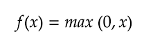
2. ReLU (Rectified Linear Unit) Activation Function: This function maps any input to a value between 0 and infinity. It is widely used in deep learning because of its simplicity and computational efficiency. Example:
   

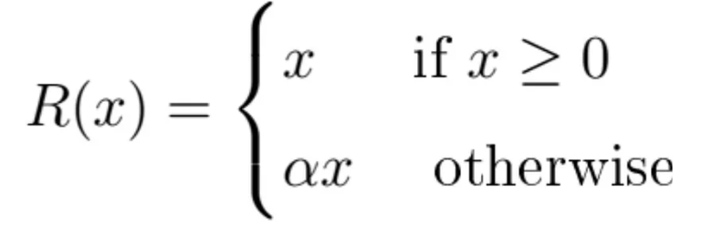
3. Leaky ReLU Activation Function: This function is similar to the ReLU function, but it allows a small negative slope for negative input values. This helps to avoid the dying ReLU problem. Example:
   

4. Tanh (Hyperbolic Tangent) Activation Function: This function maps any input to a value between -1 and 1. It is used in binary classification tasks similar to the sigmoid function. Example:

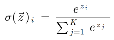
5. Softmax Activation Function: This function is used in multi-class classification tasks. It maps the output of each neuron to a value between 0 and 1, and the sum of all the outputs is equal to 1.
   

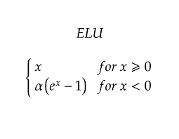
6. ELU (Exponential Linear Unit) Activation Function: This function is similar to the ReLU function, but it allows a small negative value for negative input values. Example:
   

The choice of activation function can have a significant impact on the performance of a neural network, as different functions can introduce different types of non-linearity. The goal is to choose an activation function that allows the network to learn the desired function while avoiding issues like vanishing gradients or exploding gradients.

Loss Function

A loss function, also known as a cost function or objective function, is a mathematical function that measures the difference between the predicted output of a model and the actual output. The role of the loss function in training a model is to guide the learning process by providing a measure of how well the model is performing on a given task.

The goal of training a model is to minimize the loss function, which is achieved by adjusting the weights and biases of the model during the optimization process. The loss function provides feedback to the optimizer, allowing it to make adjustments that improve the model's predictions.

There are many different types of loss functions, each suited to different types of tasks. Some common loss functions include mean squared error (MSE), cross-entropy loss, and hinge loss.

• MSE is a popular loss function for regression problems, where the goal is to predict a continuous output. It measures the average squared difference between the predicted output and the actual output.

• Cross-entropy loss is commonly used in classification tasks, where the goal is to predict a categorical output. It measures the difference between the predicted probability distribution and the true probability distribution.

• Hinge loss is commonly used in binary classification tasks, where the goal is to predict one of two possible outcomes. It measures the difference between the predicted output and the actual output, but only penalizes errors that exceed a certain threshold.

The choice of loss function depends on the specific task and the type of model being trained. Selecting an appropriate loss function is an important step in designing an effective machine learning system.

Convolution

Convolution is a fundamental operation in deep learning that involves applying a filter to an input signal to extract certain features. In the context of image processing, the input signal is a 2D or 3D image, and the filter is a small matrix called a kernel.

There are several types of convolution that are commonly used in deep learning:

• 2D Convolution: This is the most common type of convolution used in image processing, where a 2D kernel is applied to a 2D image.

• 3D Convolution: This type of convolution is used for processing 3D data such as videos or medical images, where a 3D kernel is applied to a 3D volume.

• Depthwise Convolution: This type of convolution operates on each channel of an input separately, rather than across all channels at once. It is commonly used in mobile neural networks to reduce the number of parameters and computation needed.

• Transposed Convolution: This operation is also known as "deconvolution" and is used to upsample feature maps. It applies a reverse operation to the standard convolution and can be useful for tasks such as image segmentation.

• Dilated Convolution: This type of convolution involves skipping input values in the kernel by a certain stride, which increases the receptive field of the output feature map. This can be useful for detecting larger patterns in the input image.

• Separable Convolution: This is a type of depthwise convolution followed by a pointwise convolution, which can be more computationally efficient than standard convolution while still achieving similar performance.

Convolution is a powerful tool in deep learning for extracting features from input data. There are several types of convolution, each with its own advantages and applications. Understanding these different types can help in choosing the right convolutional operation for a given task.

MatMul

MatMul is a term used in deep learning to describe the process of multiplying matrices. A matrix is a rectangular array of numbers, while a scalar is a single number. Matrices can be multiplied together by following a set of rules that involve multiplying the corresponding elements of each matrix and then summing the resulting products. The resulting matrix has the same number of rows as the first matrix and the same number of columns as the second matrix.

In deep learning, MatMul is commonly used in neural networks to perform operations between the input and weights matrices. The input matrix represents the features of the data, while the weight matrix represents the model's parameters that are learned during the training process. By multiplying the input matrix by the weight matrix, the neural network can make predictions based on the learned patterns in the data.

MatMul can be performed efficiently using specialized hardware such as graphics processing units (GPUs), which can handle large matrices with thousands or even millions of elements. This allows deep learning models to process large amounts of data quickly and accurately.

Overfitting

Overfitting is a common problem in machine learning where a model becomes too complex and fits the training data too closely. This results in a model that has high accuracy on the training data, but performs poorly on new, unseen data.

One of the causes of overfitting is when a model is too complex for the amount of data available. When there are more parameters in the model than there are training examples, the model can essentially "memorize" the training data rather than learning a generalizable pattern.

Another cause of overfitting is when the model is trained for too long, resulting in it fitting noise in the training data rather than the underlying pattern. Additionally, if the model is not regularized properly or the training data is not diverse enough, overfitting can occur.

The consequences of overfitting can be severe, as the model may perform poorly on new, unseen data. This can result in incorrect predictions, which can have negative consequences in many real-world applications.

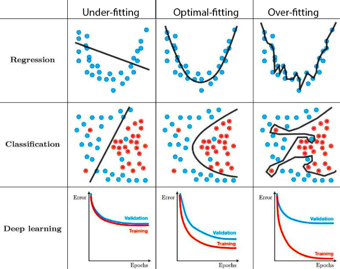
To prevent overfitting, there are several techniques that can be employed. One of the most common techniques is regularization, which adds a penalty term to the loss function to discourage overfitting. Dropout is another technique that randomly drops out nodes during training, preventing the model from relying too heavily on any one node. Finally, early stopping can be used to stop training when the model begins to overfit, preventing it from fitting noise in the training data.

Dropout

Dropout is a regularization technique used in deep learning to prevent overfitting of neural networks. Overfitting occurs when the model becomes too complex and starts fitting the training data too closely, leading to poor generalization on new data. Dropout addresses this problem by randomly dropping out some neurons during the training phase.

In dropout, a certain percentage of randomly selected neurons are ignored during each training iteration. This means that the remaining neurons must learn to compensate for the missing neurons, which helps prevent overfitting by promoting redundancy in the network. During inference, all neurons are used, but their outputs are multiplied by the probability of being active during training.

Dropout has been shown to be effective in preventing overfitting in a variety of neural network architectures, including convolutional neural networks and recurrent neural networks. By reducing overfitting, dropout can lead to improved generalization performance and better accuracy on new data.

Example of dropout:
Suppose we have a fully connected neural network with three hidden layers, each containing 100 neurons. We apply a dropout rate of 0.5, which means that during each training iteration, 50% of the neurons in each layer are randomly ignored. As a result, the remaining neurons must learn to compensate for the missing neurons, leading to a more robust network. During inference, all neurons are used, but their outputs are multiplied by 0.5, which ensures that the expected output remains the same as during training.

Early Stopping

Early stopping is a technique used to prevent overfitting in deep learning models. During training, the model is evaluated on a validation dataset, and the performance metric (such as accuracy or loss) is monitored. As training progresses, the model's performance on the validation dataset may begin to decrease, while its performance on the training dataset continues to improve. This is a sign that the model is overfitting, meaning it is becoming too specialized to the training dataset and may not generalize well to new data.

To prevent overfitting, early stopping interrupts the training process when the model's performance on the validation dataset begins to decrease. The point at which training is stopped is determined by comparing the performance on the validation dataset over multiple training epochs. The idea is to find the point at which the model achieves the best performance on the validation dataset, before its performance starts to degrade due to overfitting.

Once early stopping is triggered, the weights of the model at the point of best validation performance are saved and used as the final model. Early stopping is a simple and effective technique for preventing overfitting, and it can help to improve the generalization performance of deep learning models.

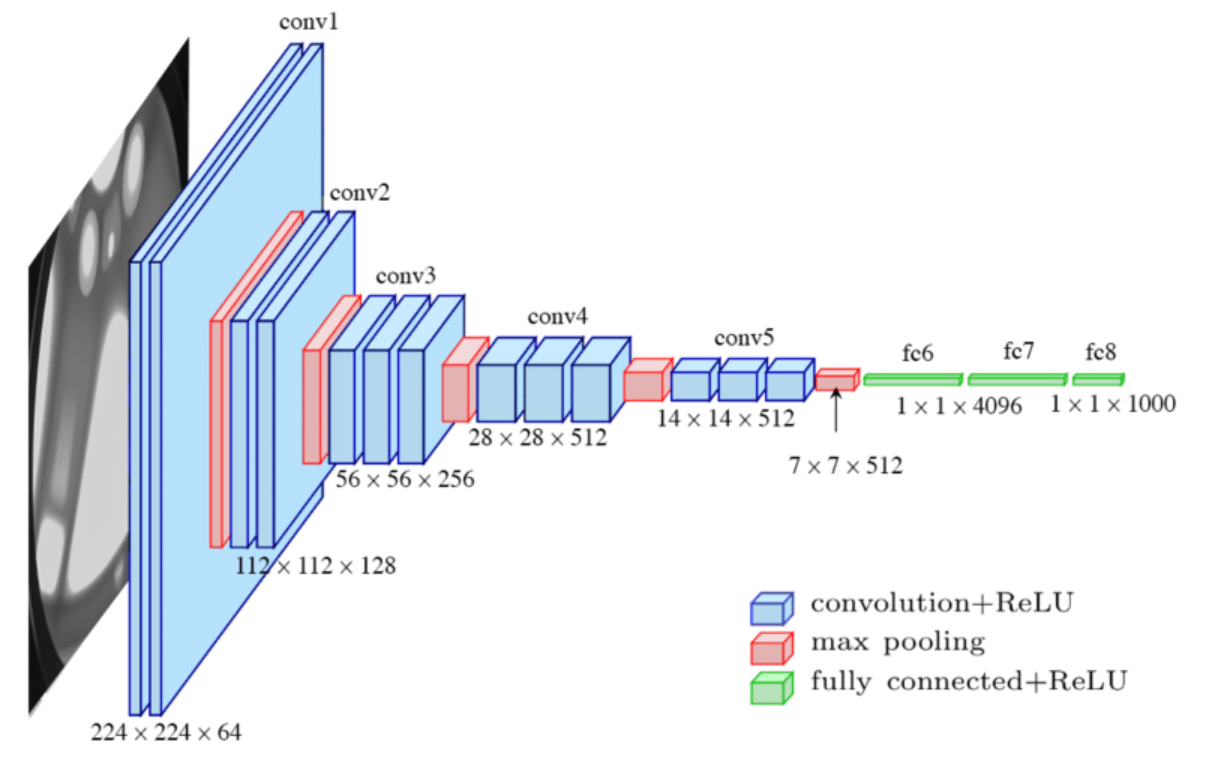
Convolutional Neural Networks (CNNs)

Convolutional Neural Networks (CNNs) are a type of deep learning model that are particularly well-suited for processing and analyzing image data. They are designed to automatically learn features from images, such as edges, textures, and shapes, which can then be used for tasks such as object detection and image classification.

At a high level, CNNs consist of several layers, including convolutional layers, pooling layers, and fully connected layers. The convolutional layers use a set of filters to extract features from the input image. Each filter is convolved with the input image to produce a feature map, which highlights areas of the image that match the filter.

The pooling layers are used to reduce the dimensionality of the feature maps, making the model more computationally efficient. The most common type of pooling is max pooling, which takes the maximum value within each sub-region of the feature map.

The fully connected layers are used to produce the final output of the model, such as a class label or a bounding box for object detection.

One of the key advantages of CNNs is their ability to learn hierarchical representations of the input data. The early layers of the network learn low-level features, such as edges and textures, while the later layers learn higher-level features, such as object parts and entire objects. This hierarchical structure allows the model to learn very complex representations of the input, which can be used for a wide range of image processing tasks.

There are many different CNN architectures, each with its own strengths and weaknesses. One example of a popular CNN architecture is the VGG network, which consists of 16 or 19 layers and has been used for tasks such as image classification and object detection.

Here are some examples of CNN models:

1. ResNet (Residual Network): ResNet is a deep CNN architecture that is designed to address the problem of vanishing gradients in deep networks. It introduced the concept of residual blocks, which allowed the network to learn residual functions instead of directly trying to learn the underlying mapping. This enabled the network to achieve better accuracy with deeper layers, up to 152 layers in the case of ResNet152.

2. MobileNet: MobileNet is a lightweight CNN architecture designed for mobile and embedded devices. It uses depthwise separable convolutions to reduce the number of parameters and operations required, making it more efficient than traditional CNNs. This makes it ideal for applications with limited computational resources.

3. GoogleNet (Inception): GoogleNet, also known as Inception, is a CNN architecture that introduced the concept of inception modules. These modules are designed to capture features at multiple scales by performing convolutions with filters of different sizes in parallel. GoogleNet also includes auxiliary classifiers to combat the problem of vanishing gradients.

In conclusion, Convolutional Neural Networks are a powerful tool for processing and analyzing image data. Their ability to automatically learn features from the input data, combined with their hierarchical structure, make them well-suited for a wide range of image processing tasks.

Pooling

Pooling is a technique used in neural networks to reduce the spatial dimensions of the feature maps generated by convolutional layers. The main purpose of pooling is to reduce the size of the feature maps, while also retaining the important features.

Pooling works by dividing the input feature map into a set of non-overlapping rectangular regions, called pooling regions, and then applying a pooling function to each region. The most commonly used pooling functions are max pooling and average pooling.

There are several types of pooling layers, including:

1. Max Pooling: Max pooling is the most commonly used pooling layer in CNNs. It operates by dividing the input image into non-overlapping rectangular regions and taking the maximum value within each region. This effectively downsamples the feature map while retaining the most salient information.

2. Average Pooling: Average pooling is similar to max pooling, but instead of taking the maximum value within each region, it takes the average. This can be useful when you want to preserve the general structure of the input image, but not necessarily the exact details.

3. Minimun Pooling: In Min Pooling, the minimum activation value within the pooling window is selected as the output value. This type of pooling can be useful in certain applications, such as anomaly detection or signal processing, where the focus is on detecting the smallest or most unusual values in a dataset.

4. Global Pooling: Global pooling, also known as global average pooling or global max pooling, applies the pooling operation to the entire feature map, rather than dividing it into regions. This results in a single value for each channel, effectively reducing the feature map to a vector. Global pooling can be useful when you want to obtain a fixed-length representation of the entire input image.

5. Lp Pooling: Lp pooling is a more general form of pooling that takes the Lp norm of the values within each region, rather than just the maximum or average. The Lp norm is a generalization of the Euclidean norm, which is used in L2 regularization. Different values of p can be used to emphasize different types of information in the feature map.

The pooling operation reduces the size of the feature maps, which in turn reduces the number of parameters in the model and helps to prevent overfitting. It also helps to make the model more robust to small variations in the input, by allowing it to recognize important features regardless of their exact location in the input.

Overall, pooling is an important technique for reducing the spatial dimensions of feature maps, while retaining the important features, and is commonly used in modern convolutional neural networks.

Flatten

Flatten is a simple operation used in deep learning that takes an input tensor with multiple dimensions and flattens it into a one-dimensional tensor. This is often necessary when passing data from one layer to another in a neural network.

For example, suppose we have an image with dimensions 28x28x3, where 28x28 is the height and width of the image and 3 represents the RGB channels. We can use the flatten operation to convert this image into a one-dimensional tensor of size 2352 (28x28x3).

Recurrent Neural Networks (RNNs)

Recurrent Neural Networks (RNNs) are a type of neural network that are designed to process sequential data, such as time series data or natural language text. Unlike feedforward neural networks, which process input data in a single pass, RNNs maintain an internal state that allows them to process sequential data one element at a time.

At a high level, an RNN consists of a set of recurrently connected neurons, where the output of each neuron is fed back into the network as input to the next time step. This feedback loop allows the network to maintain an internal state, which can be used to process sequences of variable length.

RNNs are particularly well-suited for tasks such as language modeling, where the goal is to predict the probability distribution of the next word in a sequence given the previous words. They are also commonly used for tasks such as speech recognition, machine translation, and image captioning.

One of the key advantages of RNNs is their ability to model long-term dependencies in sequential data. This is achieved through the use of the internal state, which allows the network to maintain information about previous elements in the sequence. However, RNNs can also suffer from the vanishing gradient problem, where the gradient of the loss function with respect to the weights of the network becomes very small as it is propagated back in time. This can make it difficult to train RNNs to model long-term dependencies.

There are many different RNN architectures, each with its own strengths and weaknesses. One example of a popular RNN architecture is the Long Short-Term Memory (LSTM) network, which is designed to address the vanishing gradient problem. LSTMs use a set of gating mechanisms to control the flow of information through the network, allowing it to selectively remember or forget information from previous time steps.

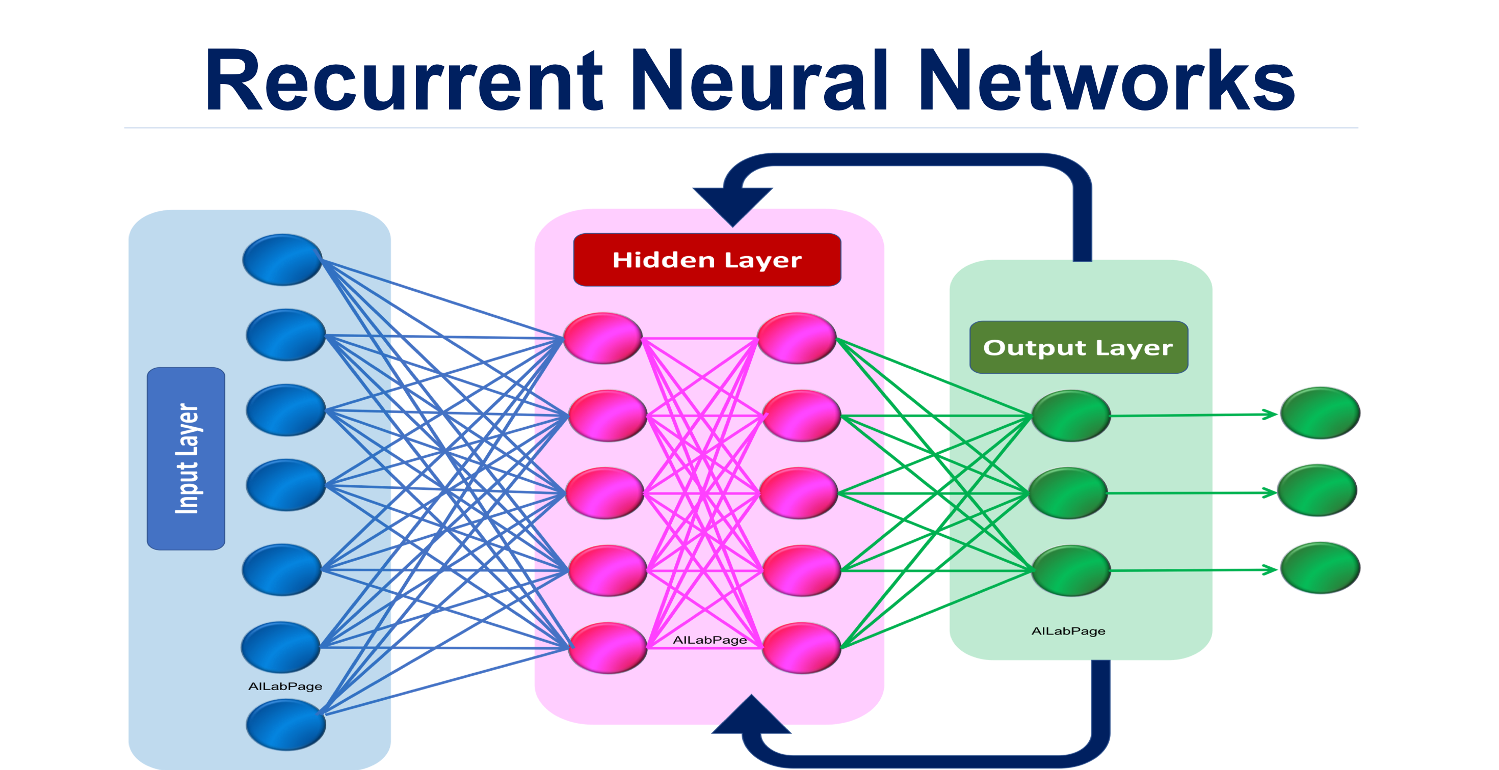
In conclusion, Recurrent Neural Networks are a powerful tool for processing sequential data. Their ability to maintain an internal state and model long-term dependencies make them well-suited for a wide range of tasks, including language modeling and speech recognition. However, their susceptibility to the vanishing gradient problem means that careful training is required to achieve good performance.

Long Short Term Memory (LSTM)

LSTM stands for Long Short-Term Memory, which is a type of recurrent neural network (RNN) that is designed to overcome the issue of vanishing gradients in traditional RNNs.

LSTMs are especially useful in sequence prediction tasks, such as natural language processing, speech recognition, and time series forecasting. The basic structure of an LSTM consists of a memory cell, an input gate, an output gate, and a forget gate.

The memory cell is the core component of an LSTM and stores information over a long period of time. The input gate controls the flow of information into the memory cell, the output gate controls the flow of information out of the memory cell, and the forget gate controls which information should be removed from the memory cell.

During training, the LSTM learns to adjust the weights of its different gates and cell state in order to optimize its performance on a given task. This training process involves backpropagation through time, which allows the LSTM to learn from previous time steps and make predictions based on the sequence of inputs.

Overall, LSTMs have proven to be a powerful tool for sequence prediction tasks due to their ability to handle long-term dependencies and avoid the issue of vanishing gradients that can occur in traditional RNNs.

Autoencoder

An autoencoder is a type of neural network that is trained to reconstruct its own inputs. It consists of two parts: an encoder and a decoder. The encoder compresses the input data into a lower-dimensional representation, also known as a latent code or embedding. The decoder then attempts to reconstruct the original input from this compressed representation.

The goal of an autoencoder is to learn a compressed representation of the input data that captures the most important features or patterns in the data. By doing so, it can be used for a variety of tasks such as dimensionality reduction, feature extraction, and data generation.

Autoencoders are trained using an unsupervised learning approach, which means that they do not require labeled data for training. The training process involves minimizing the difference between the original input and the reconstructed output, which is typically measured using a loss function such as mean squared error (MSE) or binary cross-entropy.

Autoencoders can be used for a variety of applications such as image denoising, image compression, anomaly detection, and generative modeling. Variations of autoencoders such as denoising autoencoders, variational autoencoders (VAEs), and generative adversarial networks (GANs) have been developed to improve their performance and extend their applications.

Transfer Learning

Transfer learning is a technique in machine learning where a pre-trained model is used as a starting point for a new task. In transfer learning, knowledge gained from training on one task is applied to another related task, with the goal of improving performance and reducing the amount of training data required.

The idea behind transfer learning is that pre-trained models have already learned many useful features from large amounts of data, and these features can be leveraged to accelerate training on a new task. For example, a model trained to recognize objects in photographs can be used as a starting point for a new model that recognizes specific types of objects, such as cars or animals.

Transfer learning can be especially useful when there is limited training data available for the new task, or when the new task is similar to the original task. By starting with a pre-trained model, the new model can learn from the knowledge gained by the original model, potentially reducing the amount of time and resources required for training.

An example of transfer learning in action is the use of pre-trained models in natural language processing (NLP). Many pre-trained models are available for tasks such as sentiment analysis and named entity recognition, and these models can be fine-tuned for specific applications such as chatbots or question answering systems.

In computer vision, transfer learning has also been used to improve the performance of image classification models. For example, a pre-trained model such as VGG or ResNet can be used as a starting point for a new model that recognizes specific types of objects or scenes.

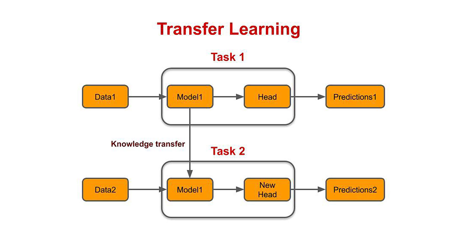
In conclusion, transfer learning is a powerful technique for improving the performance of machine learning models. By leveraging the knowledge gained by pre-trained models, transfer learning can reduce the amount of training data required and accelerate the training process. It has been successfully applied in a variety of applications, from natural language processing to computer vision.

Generative Adversarial Networks (GANs)

Generative Adversarial Networks, or GANs, are a type of deep learning model that consists of two neural networks: a generator and a discriminator. The generator network takes in random noise as input and produces a sample that is intended to be similar to the real data. The discriminator network takes in both real data and generated data as input and tries to distinguish between the two.

The training process for GANs involves training the generator and discriminator networks simultaneously in a competitive setting. The generator tries to produce realistic samples that fool the discriminator, while the discriminator tries to correctly identify whether the input is real or generated.

During training, the generator is updated based on how well it is able to fool the discriminator, while the discriminator is updated based on how well it is able to distinguish between real and generated data. This process continues until the generator is able to produce samples that are indistinguishable from real data and the discriminator is no longer able to differentiate between real and generated data.

Overall, GANs are used for generating realistic and diverse samples of data, such as images, music, or text, that can be used for various applications such as image synthesis, data augmentation, and style transfer.

Artificial Neural Networks (ANNs)

Artificial Neural Networks (ANNs) are one of the most fundamental building blocks of deep learning. ANNs are inspired by the structure and function of the human brain, consisting of layers of interconnected nodes called neurons. ANNs are used for a wide range of applications, including image recognition, natural language processing, and voice recognition.

At a high level, ANNs consist of input and output layers, with one or more hidden layers in between. The input layer takes in the data, and the output layer produces the result of the model. The hidden layers are where the majority of the processing occurs. Each neuron in a layer is connected to every neuron in the previous layer, and the connections between the neurons are assigned weights.

During the training process, the weights of the connections between neurons are adjusted to minimize a loss function. This is accomplished through a process called backpropagation, which involves propagating the error from the output layer back through the network to adjust the weights of the connections. The process is repeated multiple times until the model is able to accurately predict the output for a given input.

One of the key advantages of ANNs is their ability to learn from large amounts of data. This makes them well-suited for tasks such as image recognition and speech recognition, which require vast amounts of training data. ANNs can also be used for unsupervised learning tasks, such as clustering and dimensionality reduction.

In conclusion, Artificial Neural Networks are a powerful tool for deep learning that are used for a wide range of applications. Their ability to learn from large amounts of data, coupled with their ability to generalize to new data, make them a valuable tool for data scientists and machine learning practitioners.

Hyperparameter

Hyperparameters are parameters that are set by the user before training a machine learning model. These parameters are not learned during training, but rather are chosen by the user based on experience and trial-and-error to optimize the performance of the model.

In deep learning, there are many hyperparameters that can be tuned to improve the performance of a model. Some common hyperparameters include the learning rate, batch size, number of layers in the neural network, and the number of neurons in each layer.

The learning rate determines how quickly the model adjusts its parameters during training based on the error it makes. A larger learning rate can lead to faster convergence but may also cause the model to overshoot the optimal values, while a smaller learning rate may take longer to converge but can produce more accurate results.

The batch size determines how many training examples are used in each iteration of the model during training. A larger batch size can lead to faster training, but can also require more memory and may result in overfitting, while a smaller batch size can lead to slower training but may produce better generalization.

The number of layers and neurons in each layer can also have a significant impact on the performance of a model. A larger number of layers and neurons can potentially capture more complex patterns in the data but can also lead to overfitting and longer training times.

Hyperparameters can greatly affect the performance of a deep learning model, and finding the optimal values for each hyperparameter is often a trial-and-error process. Techniques such as grid search and random search can be used to explore the space of possible hyperparameters and find the best combination for a given task.

In summary, hyperparameters are parameters set by the user before training a model and can greatly impact the performance of a deep learning model. Common hyperparameters include the learning rate, batch size, and the number of layers and neurons in each layer and finding the optimal values for each hyperparameter is often a trial-and-error process.

Learning Rate

Learning rate is a hyperparameter that controls the step size at each iteration while updating the weights of a neural network during training. It determines how quickly or slowly the model will learn from the data. A learning rate that is too small may take too long to converge, while a learning rate that is too large may cause the model to overshoot the optimal solution and fail to converge.

The optimal learning rate varies depending on the problem and the model architecture. A common technique for tuning the learning rate is to use a learning rate schedule, which gradually decreases the learning rate over time. Another technique is to use adaptive learning rate methods such as Adam, Adagrad, or RMSprop, which adjust the learning rate based on the gradients of the weights.

It's essential to find an optimal learning rate to ensure the model converges quickly and efficiently to the optimal solution. A learning rate that's too high may cause the model to overshoot the optimal solution and fail to converge. On the other hand, a learning rate that's too low may take too long to converge, and the model may get stuck in a local minimum.

Batch Normalization

Batch normalization is a technique used in deep learning to improve the training of neural networks by normalizing the inputs to each layer. It involves normalizing the activations of a given layer by subtracting the batch mean and dividing by the batch standard deviation. This ensures that the inputs to each layer are approximately Gaussian, which can help to reduce the effects of covariate shift and improve the convergence of the training process.

During training, batch normalization operates on a minibatch of data rather than the entire dataset. This means that the mean and standard deviation used for normalization are calculated based only on the data in the current minibatch, rather than the entire dataset. This can help to regularize the training process and prevent overfitting, as the statistics used for normalization will vary from minibatch to minibatch.

Batch normalization can be applied to the inputs of a layer, as well as the outputs. In the case of the input, the batch normalization operation is applied before the activation function. In the case of the output, the batch normalization operation is applied after the activation function.

An example of batch normalization in action would be training a deep convolutional neural network for image classification. The network would be trained on a large dataset of labeled images, with batch normalization applied to each layer of the network. The batch normalization operation would help to ensure that the inputs to each layer are normalized, which can improve the convergence of the training process and help to prevent overfitting. The resulting network would be better able to generalize to new images and achieve higher accuracy on the classification task.

Quantization

Quantization is the process of reducing the number of bits required to represent a numerical value, while minimizing the loss of information. In the context of deep learning, quantization refers to the process of reducing the precision of weights and activations in neural networks.

Traditional neural networks typically use 32-bit floating-point numbers to represent weights and activations, which can be computationally expensive and memory-intensive. Quantization techniques can be used to represent these values using smaller, fixed-point numbers, such as 8-bit integers.

Quantization can help to reduce the memory footprint of neural networks, making them more efficient for deployment on resource-constrained devices such as mobile phones or embedded systems. However, quantization can also introduce some loss of accuracy in the network's predictions, especially if not done carefully. Therefore, it is important to carefully tune the quantization parameters to balance the trade-off between model size and accuracy.

Inference

Inference is the process of using a trained machine learning model to make predictions on new, unseen data. After a machine learning model has been trained on a dataset, it can be used to make predictions on new data points that were not part of the training set.

During inference, the input data is fed into the trained model, which processes the data and produces an output. The output could be a single number, a vector, or a sequence of values, depending on the specific task that the model was trained to perform. For example, a trained image classification model might take an input image and output a label indicating the most likely category for that image.

Inference can be performed using the same programming language and tools that were used to train the model. In many cases, the trained model can be loaded into memory and called from a script or application to make predictions on new data.

Here are several types of inference that can be used in deep learning, depending on the specific use case and hardware constraints. Here are some examples:

• Forward Inference: This is the most common type of inference and involves running the model forward through the neural network to make a prediction based on the input data.

• Backward Inference: This type of inference is used in backpropagation, which is a method of training the neural network by adjusting the weights based on the error in the output.

• Batch Inference: This type of inference involves processing multiple inputs simultaneously in batches, which can be more efficient than processing them one at a time.

• Streaming Inference: This type of inference involves processing data in real-time as it becomes available, such as in video or audio streams.

• Edge Inference: This type of inference involves deploying the model on edge devices, such as smartphones or IoT devices, to perform inference locally without the need for a connection to the cloud.

• Cloud Inference: This type of inference involves deploying the model on cloud-based servers, which can provide greater processing power and scalability.

Each type of inference has its own advantages and disadvantages, and choosing the right one depends on the specific use case and hardware constraints.

An example of inference in action would be using a trained natural language processing (NLP) model to classify the sentiment of a text message. The model would have been trained on a large dataset of labeled text messages and would be able to classify new messages as positive, negative, or neutral based on the words and phrases in the message. To perform inference, the new text message would be fed into the trained model, which would output the predicted sentiment category. The predicted category could then be used to inform a decision or trigger an action, such as responding to the message or routing it to a specific department for further processing.

Softmax

Softmax is an activation function that is commonly used in neural networks to convert the output of a model into a probability distribution. In other words, Softmax takes a vector of raw output values and transforms it into a vector of values between 0 and 1 that sum up to 1, which can be interpreted as the probabilities of the input belonging to each class.

The Softmax function takes the form of:

Where z is the vector of raw output values from the model, and i and k represent the classes in the classification task, with K being the total number of classes.

In a classification task, the output of the Softmax function can be interpreted as the probability of the input belonging to each class. For example, if a Softmax output for a three-class classification task was [0.3, 0.5, 0.2], it can be interpreted as a 30% probability of belonging to the first class, 50% to the second class, and 20% to the third class.

The Softmax function is often used as the output layer activation function for multi-class classification tasks in neural networks. It is especially useful in cases where there are more than two classes, as it provides a probability distribution over all the classes.

Overall, the Softmax function helps to provide a probabilistic interpretation of the model's output, which can be useful in many applications, such as natural language processing and computer vision.

Natural Language Processing(NLP)

NLP stands for Natural Language Processing, which is a branch of Artificial Intelligence (AI) that deals with the interaction between computers and human languages. NLP enables computers to read, understand, interpret, and generate natural human language.

NLP is used in various applications such as chatbots, sentiment analysis, machine translation, speech recognition, and text summarization. The core techniques used in NLP include tokenization, part-of-speech tagging, parsing, named entity recognition, sentiment analysis, machine learning, and deep learning.

Machine learning and deep learning are used in NLP to build models that can learn from data and make predictions. The most popular deep learning models used in NLP are Recurrent Neural Networks (RNNs), Convolutional Neural Networks (CNNs), and Transformers. These models have been used to achieve state-of-the-art results in various NLP tasks, such as machine translation, text classification, and question-answering systems.

Two of the most popular NLP models that have been developed in recent years are GPT and BERT. The Generative Pretrained Transformer (GPT) model was developed by OpenAI and is designed to generate natural language text. It uses a deep neural network architecture called the Transformer, which was first introduced in a research paper by Google in 2017. The GPT model is trained on a large corpus of text data, such as Wikipedia articles, and is then fine-tuned on specific tasks, such as language translation or text completion.

BERT, which stands for Bidirectional Encoder Representations from Transformers, is another NLP model that has gained a lot of attention in recent years. BERT was also developed by Google and is designed to perform tasks such as language understanding, sentiment analysis, and question answering. BERT is a pre-trained model that uses a technique called masked language modeling, where certain words in a sentence are randomly replaced with a "mask" token and the model is then trained to predict the correct word. BERT also uses the Transformer architecture and is capable of processing large amounts of text data.

Other popular NLP models include Transformer-XL, ELMo, and ULMFiT. These models are designed to perform a range of NLP tasks, from language translation to text classification. Each of these models uses different techniques and architectures to achieve high levels of accuracy on specific NLP tasks.

Overall, NLP plays a vital role in bridging the gap between humans and computers by enabling computers to understand and generate human language, which has a wide range of practical applications in various fields.

Tokenization

Tokenization is a common natural language processing technique used to split up text into smaller meaningful units called tokens. In NLP, these tokens can be words, phrases, or even individual characters. Tokenization is an essential step in text processing as it allows machines to better understand and analyze natural language data.

The process of tokenization can vary depending on the application, but typically involves splitting the input text based on certain rules or patterns. For example, in word-level tokenization, the text is split into individual words based on spaces or punctuation marks. In character-level tokenization, the text is split into individual characters.

Tokenization can be useful in a variety of NLP tasks, such as text classification, sentiment analysis, and machine translation. By breaking down text into smaller units, machines can more easily process and analyze natural language data, leading to more accurate and effective results.

Word Embeddings

Word embeddings are a technique used in natural language processing (NLP) to represent words as numerical vectors in a high-dimensional space. The idea behind word embeddings is to capture the meaning and semantic relationships between words in a language, and to represent this information in a way that can be used by machine learning algorithms.

The basic idea is that each word is represented by a vector in a high-dimensional space, where each dimension represents a different feature or characteristic of the word. The values in each dimension of the vector represent how strongly the word exhibits that feature. For example, the vector for the word "king" might have high values in dimensions that represent masculinity, royalty, and power.

Word embeddings are usually learned from large amounts of text data using techniques like Word2Vec, GloVe, or fastText. These algorithms use unsupervised learning techniques to learn the embedding vectors that best capture the relationships between words in the training data. Once the word embeddings have been learned, they can be used as input to a wide variety of NLP tasks, such as sentiment analysis, text classification, and machine translation.

One of the key benefits of word embeddings is that they allow machine learning algorithms to work with text data in a more structured and meaningful way. Rather than simply treating words as arbitrary strings of characters, word embeddings provide a way to represent the meaning and relationships between words in a way that can be used for downstream NLP tasks.

Supervised Learning

Supervised learning is a type of machine learning where the algorithm is trained using labeled data. Labeled data means that the input data and the corresponding output data are given to the algorithm during the training phase. The goal of supervised learning is to learn a mapping function from input data to output data, so that when new input data is given to the algorithm, it can predict the corresponding output data.

For example, in a spam email detection system, the algorithm is trained using a dataset of emails, where each email is labeled as spam or not spam. The algorithm learns from this labeled data to identify patterns in the emails that distinguish spam from non-spam emails. When a new email is given to the algorithm, it predicts whether the email is spam or not based on what it has learned from the labeled data.

Supervised learning is used in many applications, such as image recognition, speech recognition, natural language processing, and recommendation systems.

• Training Dataset: The training dataset is used to train our model on the task at hand. During the training process, the model learns from the input data and the corresponding output labels. We iterate through the training dataset multiple times (epochs) to improve the model's performance.

• Validation Dataset: The validation dataset is used to tune the hyperparameters of our model, such as the learning rate or the number of layers. We use the validation dataset to evaluate the performance of the model on data that it has not seen during the training phase. This helps us avoid overfitting our model to the training data.

• Test Dataset: The test dataset is used to evaluate the final performance of our model. We evaluate our model on the test dataset after we have trained and tuned it using the training and validation datasets. The test dataset is essential to ensure that our model is able to generalize well to new, unseen data.

Unsupervised Learning

Unsupervised learning is a type of machine learning where the algorithm learns from data without any specific labels or targets to predict. Instead, the algorithm tries to find patterns and relationships within the data on its own. In other words, the algorithm is given a dataset and is expected to find meaningful structures or groupings in the data without being told what those structures or groupings are.

For example, imagine you have a dataset of customer transactions at a grocery store. In unsupervised learning, the algorithm would analyze the data to identify patterns and groupings that might not be immediately obvious. It might find that certain items tend to be purchased together, or that certain groups of customers tend to buy certain types of products. These insights could then be used to inform business decisions, such as how to optimize store layouts or how to target certain customer groups with specific promotions.

Unsupervised learning algorithms can be used for a variety of tasks, including clustering, anomaly detection, and dimensionality reduction. Some common techniques used in unsupervised learning include k-means clustering, principal component analysis (PCA), and autoencoders.

Reinforcement learning

Reinforcement learning is a type of machine learning where an agent learns to take actions in an environment to maximize a cumulative reward. The agent interacts with the environment by taking actions, and the environment responds with rewards and new states. The goal of the agent is to learn a policy, which is a mapping of states to actions, that maximizes the expected cumulative reward over time.

In reinforcement learning, the agent doesn't receive labeled examples like in supervised learning. Instead, the agent learns from trial and error by exploring the environment and trying different actions to see which ones result in the highest reward. Reinforcement learning is used in various applications, such as game playing, robotics, and control systems.

Conclusion

In conclusion, deep learning is a powerful approach to machine learning that has become increasingly popular in recent years. It involves the use of artificial neural networks, which are structured similarly to the human brain, and are trained to make predictions or classifications based on input data.

By learning and applying these key terms, you can start to explore the exciting world of deep learning and its many applications.