
Reading time: 20 minutes
The perceptron was invented in 1957 by Frank Rosenblatt and sought to binary classify an input data. It was inspired by the ability of the central nervous system of the humans to be able to do the tasks that we do. The perceptron was one of the building blocks of modern artificial intelligence as we know it today. It is the basis of the neural networks that we use to carry out a multitude of complex calculations and help computers try to mimic the human brain. In this article we will be diving into various algorithms that make the perceptron carry out binary classification.
The Neuron
A perceptron is an artificial neuron that essentially:
- receives input from an input layer
- processes the input with the help of an activation function (the Heaviside step function)
- gives out the output in the form of either a 0 or a 1.
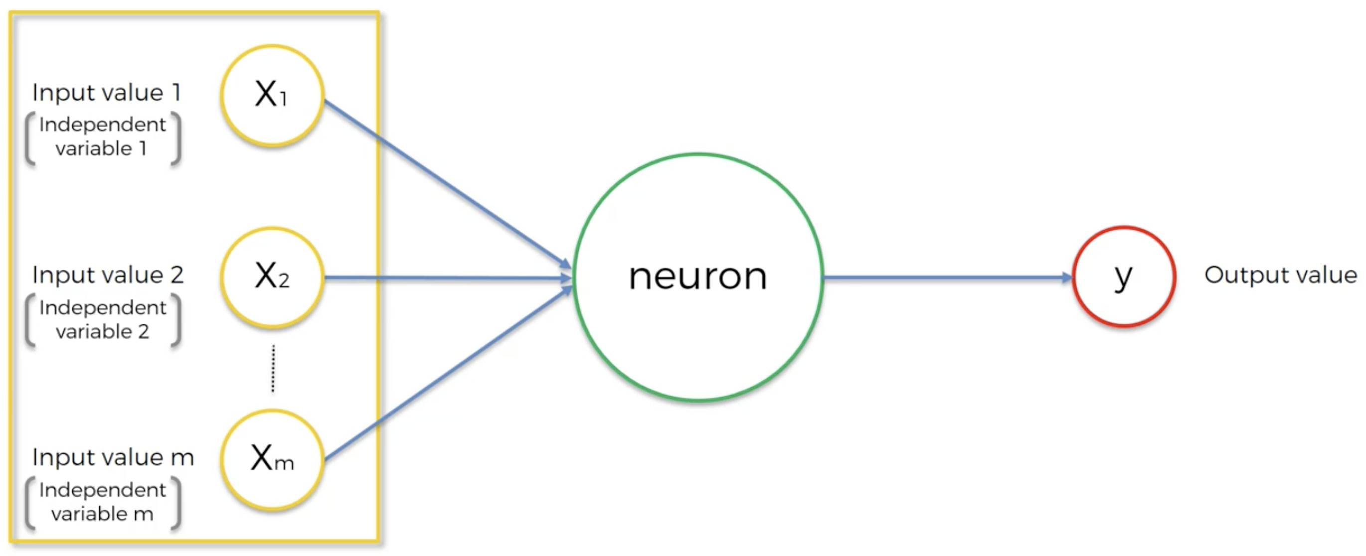
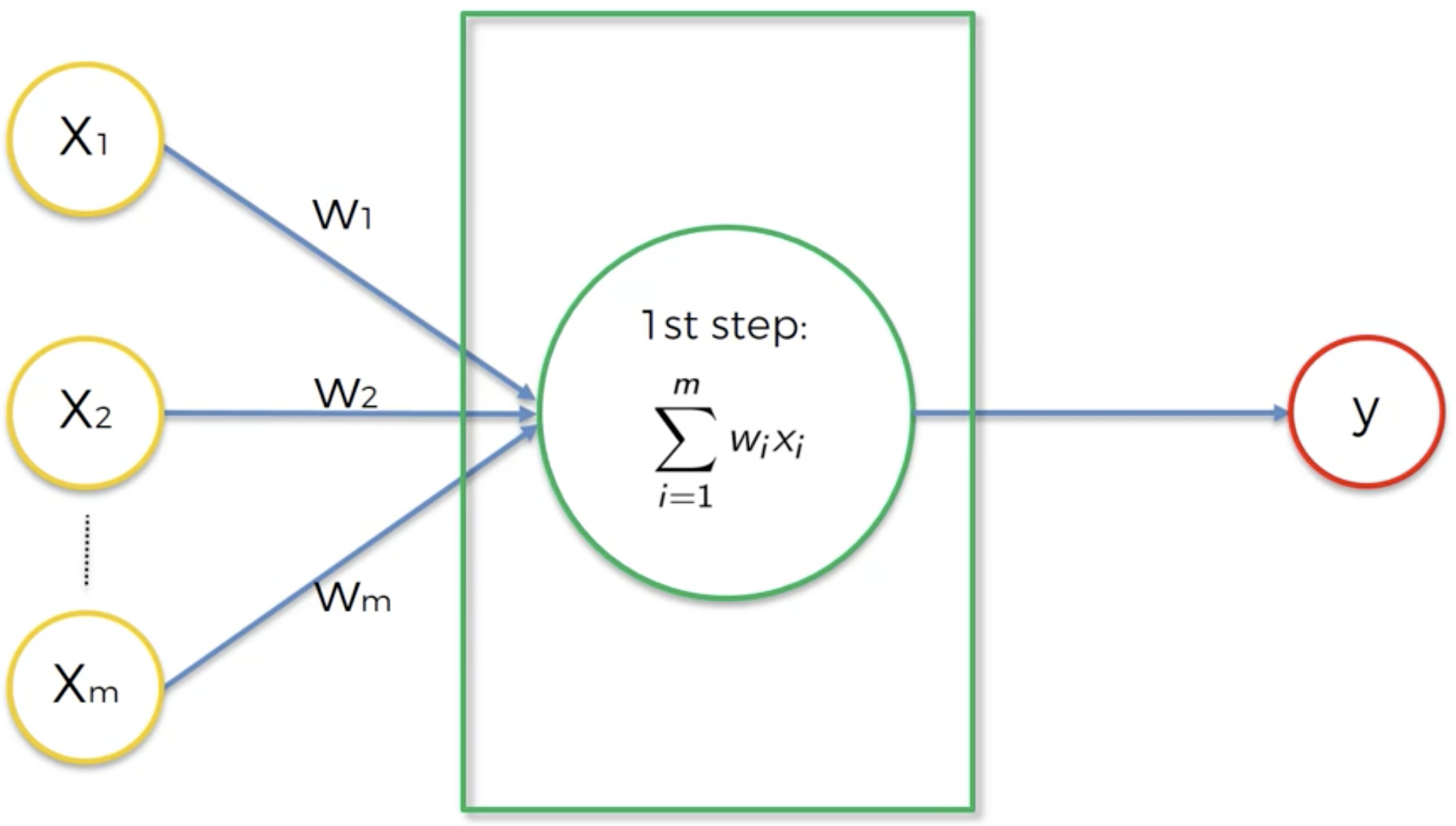
Each synapse (connection between two neurons) is assigned a weight that determines which signal is important and which is not. Once these synapses or signals enter the neuron, it does two things:
- Adds each of the product of weights and input variables
- Applies the activation function on the result of the first step
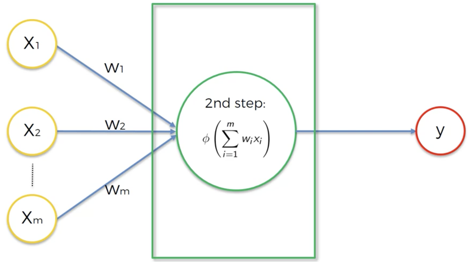
In a traditional perceptron, this activation function is the Heaviside step function (a.k.a the Unit step function or a variation of the Threshold function). It gives an output 0 if the input is less than 0 and an output 1 if the input is greater than or equal to 0. So it is easily able to classify the input variables into two categories.
However, we can use more sophisticated activation functions like the sigmoid function which would give the probabilities of the different variables existing in either category.
Weights and Back-Propagation
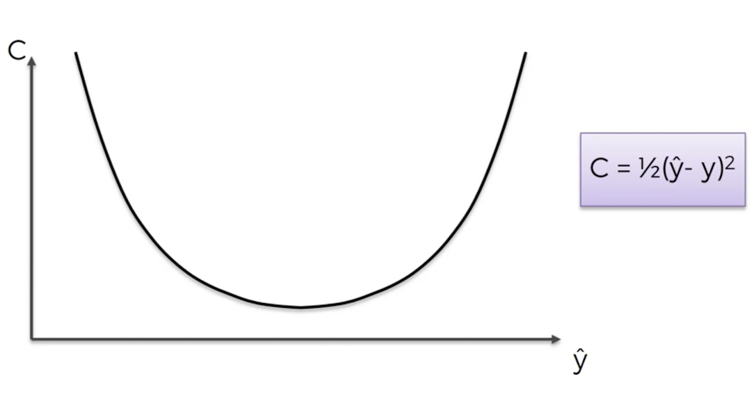
The only parameters that are autogenerated are the weights assigned to the synapses. Thus, a weight is the only parameter on which the correctness of the output depends. Very intuitively, the perceptron renders the output, "checks" the "difference" between the rendered output and the actual output, and updates the weights in the synapses accordingly. It does this as long as the "difference" between the rendered output and the actual output is minimised. The "difference" between the rendered output and the actual output is called the "cost function" and may not necessarily be the simple difference between the two but much rather is a function that compares the two. This entire process of comparison of outputs and updating weights is called back-propagation.
How to Back-Propagate: Stochastic Gradient Descent
Mathematically, we need to find the minimum value of the cost function in order to generate the most accurate output. So the following steps can be considered:
-
Start at a random point on the cost function
-
Find the derivative of the cost function
-
Repeat step 4 until the derivative is equal to 0
-
If the derivative is less than 0, move to the right i.e. y should be greater than current y, else if the derivative is greater than 0, move to the left i.e. y should be less than current y.
Once the derivative of the cost function becomes equal to 0 we know that we have reached the minimum of the cost function. This process is called the Gradient Descent since the gradient (slope of the function, derivative) is descending until it reaches 0.
However, the cost function may not always have only one minimum as shown above. It may be such that the cost function has a global minimum and many local minima. In that case, following the above steps might lead us to reach a local minimum whereas we'd get the best results at the global minimum. Hence a better way to reach to the minimum is the Stochastic Gradient Descent.
In the normal Gradient Descent, we took the entirety of our data, got the cost function and then carried out back-propagation. However, in Stochastic Gradient Descent, we take the first row of the data, render the output, back-propagate and then move on to the second row, carry out the steps, and move on to subsequent rows. This way, we reach the optimum value. So essentially, in normal Gradient Descent method, we took the bulk data together but in Stochastic Gradient Descent we take one row at a time and back-propagate.
Training a Perceptron using Stochastic Gradient Descent
To wrap things up, we compile all that is discussed above into steps that need to be carried out to train a perceptron using Stochastic Gradient Descent.
-
Initialise random weights to values close to 0 (but not 0).
-
Input first row of dataset into the input layer, with each variable assigned to each node of the layer.
-
Forward Propagation: Information flows from left to right. In the neuron, input values are multiplied with their corresponding weights and the products are added, thereafter the activation function acts on this sum of products and renders the output.
-
Compare the rendered output to the actual result and measure the generated error.
-
Back-Propagation: Information flows from right to left. Weights are updated by how much they are responsible for the error and the learning rate decides by how much we update the weights.
-
Repeat steps 1 through 5 and update the weights after each observation (Reinforcement Learning) or update the weights after a batch of observations (Batch Learning).
-
When the whole training set is passed through the perceptron, it is called an epoch. Redo more epochs.
Implementations
Below shown is the implementation of a perceptron in Python3.
Python
# Function that essentially involves the calculation inside the perceptron
def predict(row, weights):
	activation = weights[0]
	for i in range(len(row)-1):
		activation += weights[i + 1] * row[i]
	return 1.0 if activation >= 0.0 else 0.0

# Stochastic Gradient Descent
def train_weights(train, l_rate, n_epoch):
	weights = [0.0 for i in range(len(train[0]))]
	for epoch in range(n_epoch):
		sum_error = 0.0
		for row in train:
			prediction = predict(row, weights)
			error = row[-1] - prediction
			sum_error += error**2
			weights[0] = weights[0] + l_rate * error
			for i in range(len(row)-1):
				weights[i + 1] = weights[i + 1] + l_rate * error * row[i]
		print('epoch=%d, lrate=%.3f, error=%.3f' % (epoch, l_rate, sum_error))
	return weights

dataset = [[2.7810836,2.550537003,0],
	[1.465489372,2.362125076,0],
	[3.396561688,4.400293529,0],
	[1.38807019,1.850220317,0],
	[3.06407232,3.005305973,0],
	[7.627531214,2.759262235,1],
	[5.332441248,2.088626775,1],
	[6.922596716,1.77106367,1],
	[8.675418651,-0.242068655,1],
	[7.673756466,3.508563011,1]]
l_rate = 0.1
n_epoch = 5
weights = train_weights(dataset, l_rate, n_epoch)
print(weights)