Restricted Boltzmann Machines

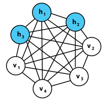
Boltzmann Machines are bidirectionally connected networks of stochastic processing units, i.e. units that carry out randomly determined processes.

A Boltzmann Machine can be used to learn important aspects of an unknown probability distribution based on samples from the distribution. Generally, this learning problem is quite difficult and time consuming. However, the learning problem can be simplified by introducing restrictions on a Boltzmann Machine, hence why, it is called a Restricted Boltzmann Machine.

Energy Based Model

Consider a room filled with gas that is homogenously spread out inside it.

Statistically, it is possible for the gas to cluster up in one specific area of the room. However, the probability for the gas to exist in that state is low since the energy associated with that state is very high. The gas tends to exist in the lowest possible energy state, i.e. being spread out throughout the room.

In a Boltzmann Machine, energy is defined through weights in the synapses (connections between the nodes) and once the weights are set, the system tries to find the lowest energy state for itself by minimising the weights (and in case of an RBM, the biases as well).

Restrictions in a Boltzmann Machine

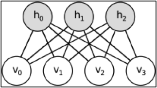
In general, a Boltzmann Machine has a number of visible nodes, hidden nodes and synapses connecting them. However, in a Restricted Boltzmann Machine (henceforth RBM), a visible node is connected to all the hidden nodes and none of the other visible nodes, and vice versa. This is essentially the restriction in an RBM.

Each node is a centre of computation that processes its input and makes randomly determined or stochastic decisions about whether to transmit the decision or not. Each visible node takes a low-level feature from the dataset to learn. E.g. in case of a picture, each visible node represents a pixel(say x) of the picture. Each value in the visible layer is processed (i.e. multiplied by the corresponding weights and all the products added) and transfered to the hidden layer. In the hidden layer, a bias b is added to the sum of products of weights and inputs, and the result is put into an activation function. This result is the output of the hidden node.

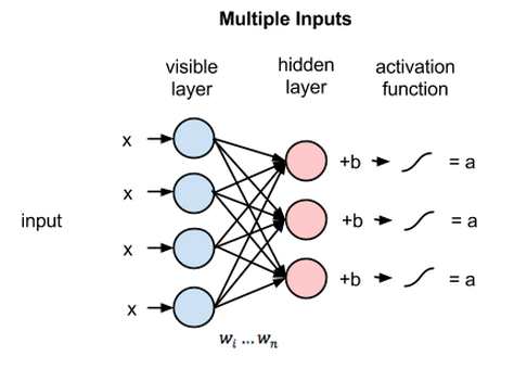
This entire process is refered to as the forward pass. Once the forward pass is over, the RBM tries to reconstruct the visible layer.

During the backward pass or the reconstruction phase, the outputs of the hidden layer become the inputs of the visible layer. Each value in the hidden node is weight adjusted according to the corresponding synapse weight (i.e. hidden node values are multiplied by their corresponding weights and the products are added) and the result is added to a visible layer bias at each visible node. This output is the reconstruction.

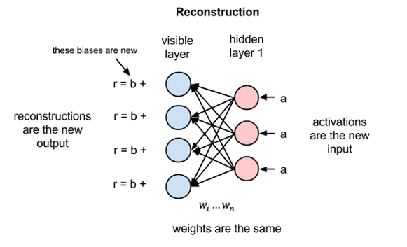
The error generated (difference between the reconstructed visible layer and the input values) is backpropagated many times until a minimum error is reached.

Gibbs Sampling

Since all operations in the RBM are stochastic, we randomly sample values during finding the values of the visible and hidden layers. For RBM's we use a sampling method called Gibbs Sampling.

1. Take the value of input vector x and set it as the value for input (visible) layer.

2. Sample the value of the hidden nodes conditioned on observing the value of the visible layer i.e. p(h|x).
   Since each node is conditionally independent, we can carry out Bernoulli Sampling i.e. if the probability of hidden node being 1 given the visible node is greater than a random value sampled from a uniform distribution between 0 and 1, then the hidden node can be assigned the value 1, else 0.
   Mathematically, 1 { p(h = 1|x) > U[0, 1] }.

3. Reconstruct the visible layer by sampling from p(x|h).

4. Repeat steps 2 and 3, k times.

Contrastive Divergence

In the case of an RBM, we take the cost function or the error as the average negative log likelihood. To minimise the average negative log likelihood, we proceed through the Stochastic Gradient Descent method and first find the slope of the cost function:

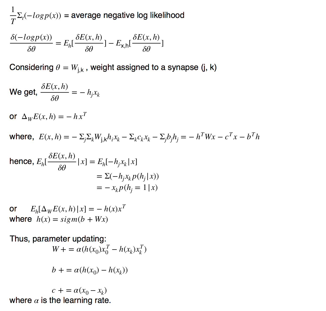
Therefore:

1. For each training example x, follow steps 2 and 3.

2. Generate x(k) using k steps of Gibbs Sampling starting at x(0).

3. Update the parameters as shown in the derivation.

4. Repeat the above steps until stopping criteria satisfies (change in parameters is not very significant etc)

For feature extraction and pre-training k = 1 works well.

Applications

RBMs have applications in many fields like:

• dimensionality reduction
• classification
• feature learning
• topic modelling
• recommender systems
• music generating

and others

More recently, Boltzmann Machines have found applications in quantum computing.

In computer vision, there are the Boltzmann Encoded Adversarial Machines which integrate RBMs and convolutional neural networks as a generative model.