We shall be discussing Gradient Ascent.

Table of Contents:

1. Gradient Ascent (Concept Explanation)
2. Application of Gradient Ascent
3. Differences with Gradient Descent

Gradient Ascent (Concept Explanation)

Gradient Ascent as a concept transcends machine learning. It is the reverse of Gradient Descent, another common concept used in machine learning. Gradient Ascent (resp. Descent) is an iterative optimization algorithm used for finding a local maximum (resp. minimum) of a function. Taking repeated steps in the direction of the gradient of the function at the current point, which is the direction of steepest ascent, invariably leads to a local maximum of the function.

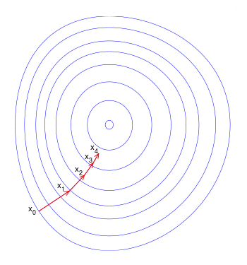
A common analogy that defines the intuition behind the application of gradient ascent algorithm to get to the local maximum is that of a hiker trying to get to the top of a mountain on a foggy day when visibility is very low. This hiker can only make his way to the mountain top by 'feeling' his path forward. A logical process the hiker can follow is to use his feet to feel the way in all directions from his current spot and determine which one has the steepest slope leading upwards and then take a small step in that direction. The hiker stops again and repeats the same thing. If this process is repeated after every step, it is guaranteed to lead the hiker to at least a local peak of the mountain. In case of convex functions which are encountered in mathematics, this is guaranteed to lead to a global maximum. The hiker's path to the top may look something like the image below:

In mathematical terms, the direction of greatest increase in slope of a function, f, is given by the gradient of that function, which is represented as \(\nabla f \). The point p at which the gradient is to be evaluated can be written as \(p=(x_{1},\ldots ,x_{n})\) in n-dimensional space so the gradient is evaluated as:
$$ \nabla f = \frac {\partial f}{\partial x_1} \hat{e_1} + \ldots + \frac {\partial f}{\partial x_n} \hat{e_n} $$
where \(\hat{e_1} ,\ldots ,\hat{e_n} \) are the unit vectors in the orthogonal directions of the n-dimensional space.

When the direction of steepest accent is known, the next thing is to take a step in that direction which mathematically translates to:
$$ y_{n+1} = y_{n} + \gamma \nabla f(y_{n}) $$
This process is repeated iteratively. \(\gamma \) is the learning rate and it determines how much step is taken by the algorithm in the direction of the gradient. A moderate learning rate is recommended.

Application of Gradient Ascent

Gradient ascent finds use in Logistic Regression. Logistic regression is a supervised Machine Learning algorithm that is commonly used for prediction and classification problems. It estimates the probability of an event occurring based on a given dataset of independent variables by computing the log-odds for the event as a linear combination of one or more independent variables. The standard logistic function \( \hat{\sigma} :\mathbb {R} \rightarrow (0,1) \) which in binary classsification maps to 0-1 classes or True-False classes is defined as:
$$ \hat{\sigma} (t) = \frac {1}{1+e^{-t}} $$
\(t\) is assumed to be a linear function of the features \(x_1,\ldots ,x_n\) as follows:
$$ t = \beta_0 + \beta_1 x_1 + \ldots + \beta_n x_n $$

The aim is to estimate the best values for the beta coefficients that maximize the model parameter called the maximum likelihood estimation (MLE). This is where the use gradient ascent method comes into play and can help determine the best fit values that will maximize the log likelihood function.
Sometimes, the negative of this function is used as the cost function and in that case, the aim will be to minimize this 'loss' and the algorithm to use in this case will be gradient descent.
The cost function to be minimized for a binary classification case is given as:
$$ \min_{w} C \sum_{i=1}^n \left(-y_i \log(\hat{\sigma}(X_i)) - (1 - y_i) \log(1 - \hat{\sigma}(X_i))\right) + r(w). $$
\(r(w)\) is the regularization term while \(y_i\) is the corresponding prediction for observation \(X_i\).

When the optimal coefficients have been found, the conditional probabilities for each observation can be calculated to give a predicted probability. For binary classification, a probability less than 0.5 will predict 0 while a probability greater than 0 will predict 1.

Differences with Gradient Descent

The main difference between gradient ascent and gradient descent is the goal of the optimization. In gradient ascent, the goal is to maximize the function while in gradient descent, the goal is to minimize the function. As a result, while both of them rely on the gradient \(\nabla f\) of the function to get the direction of steepest slope, gradient ascent takes steps in the direction of the steepest slope while gradient descent takes steps in the opposite direction. As a result, the iterative update rule for each step of the algorithm thus becomes:
$$ y_{n+1} = y_{n} + \gamma \nabla f(y_{n}) $$ for gradient ascent
and
$$ y_{n+1} = y_{n} - \gamma \nabla f(y_{n}) $$ for gradient descent