In this article, we will discover various CNN (Convolutional Neural Network) models, it's architecture as well as its uses. Go through the list of CNN models.

Table of Contents:

1. Introduction & Quick Overview about CNN.
2. Types of CNN Models.
   2.1 LeNet
   2.2 AlexNet
   2.3 ResNet
   2.4 GoogleNet/InceptionNet
   2.5 MobileNetV1
   2.6 ZfNet
   2.7 Depth based CNNs
   2.8 Highway Networks
   2.9 Wide ResNet
   2.10 VGG
   2.11 PolyNet
   2.12 Inception v2
   2.13 Inception v3 V4 and Inception-ResNet.
   2.14 DenseNet
   2.15 Pyramidal Net
   2.16 Xception
   2.17 Channel Boosted CNN using TL
   2.18 Residual Attention NN
   2.19 Attention Based CNNS
   2.20 Feautre-Map based CNNS
   2.21 Squeeze and Excitation Networks
   2.22 Competitive Squeeze and Excitation Networks

Prerequisites:

• Convolutional Neural Networks (CNN)
• Convolutional Neural Network (CNN) questions
• Disadvantages of CNN models
• When to use Convolutional Neural Networks (CNN)?

Introduction:

Convolutional Neural Networks (CNNs) are a type of Neural Network that has excelled in a number of contests involving Computer Vision and Image Processing. Image Classification and Segmentation, Object Detection, Video Processing, Natural Language Processing, and Speech Recognition are just a few of CNN's fascinating application areas. Deep CNN's great learning capacity is due to the utilisation of many feature extraction stages that can learn representations from data automatically.

The capacity of CNN to utilise spatial or temporal correlation in data is one of its most appealing features. CNN is separated into numerous learning stages, each of which consists of a mix of convolutional layers, nonlinear processing units, and subsampling layers. CNN is a feedforward multilayered hierarchical network in which each layer conducts several transformations using a bank of convolutional kernels. The convolution procedure aids in the extraction of valuable characteristics from data points that are spatially connected.

So now, since we have an idea about Convolutional Neural Networks, let’s look at different types of CNN Models.

Different types of CNN models:

1. LeNet:

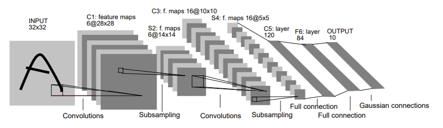
LeNet is the most popular CNN architecture it is also the first CNN model which came in the year 1998. LeNet was originally developed to categorise handwritten digits from 0–9 of the MNIST Dataset. It is made up of seven layers, each with its own set of trainable parameters. It accepts a 32 × 32 pixel picture, which is rather huge in comparison to the images in the data sets used to train the network. RELU is the activation function that has been used. The layers are laid out in the following order:

• The First Convolutional Layer is made up of 6 5 X 5 filters with a stride of 1.
• The Second Layer is a 2 X 2 average-pooling or "sub-sampling" layer with a stride of 2.
• The Third Layer is similarly a Convolutional layer, with 16 ,5 X 5 filters and a stride of 1.
• The Fourth Layer is another 2 X 2 average-pooling layer with a stride of 2.
• The fifth layer is basically connecting the output of the fourth layer with a fully connected layer consisting of 120 nodes.
• The Sixth Layer is a similarly fully-connected layer with 84 nodes that derives from the outputs of the Fifth Layer's 120 nodes.
• The seventh layer consists of categorising the output of the previous layer into ten classifications based on the 10-digits it was trained to identify.

It was one of the first effective digit-recognition algorithms for classifying handwritten digits. However, this network was ineffective in terms of computing cost and accuracy when it came to processing huge images and categorising among a large number of object classes.

2. AlexNet:

Starting with an 11x11 kernel, Alexnet is built up of 5 conv layers. For the three massive linear layers, it was the first design to use max-pooling layers, ReLu activation functions, and dropout. The network was used to classify images into 1000 different categories.

The network is similar to the LeNet Architecture, but it includes a lot more filters than the original LeNet, allowing it to categorise a lot more objects. Furthermore, it deals with overfitting by using "dropout" rather than regularisation.

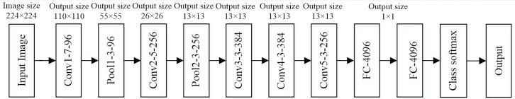
Basic layout of AlexNet architecture showing its five convolution and three fully connected layers:

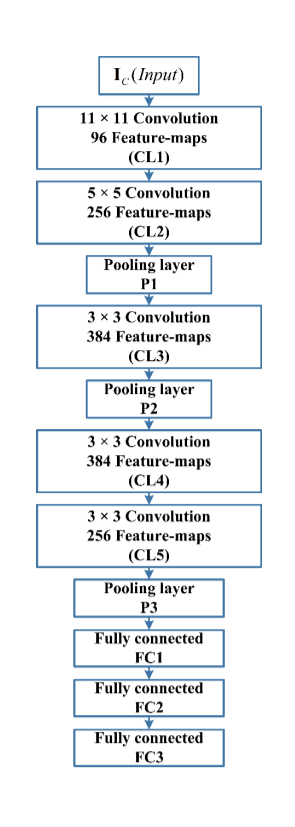
• First, a Convolution Layer (CL) with 96 11 X 11 filters and a stride of 4.
• After that, a Max-Pooling Layer (M-PL) with a filter size of 3 X 3 and a stride of 2 is applied.
• A CL of 256 filters of size 5 X 5 and stride = 4 is used once more.
• Then an M-PL with a filter size of 3 X 3 and a stride of 2 was used.
• A CL of 384 filters of size 3 X 3 and stride = 4 was used.
• Again, a CL of 384 filters of size 3 X 3 and stride = 4.
• A CL of 256 filters of size 3 X 3 and stride = 4 was used again.
• Then an M-Pl with a filter size of 3 X 3 and a stride of 2 was used.
• When the output of the last layer is transformed to an input layer, as in the Fully Linked Block, it has 9261 nodes, all of which are fully connected to a hidden layer with 4096 nodes.
• The first hidden layer is once again fully linked to a 4096-node hidden layer.

Two GPUs were used to train the initial network. It contains eight layers, each with its own set of settings that may be learned. RGB photos are used as input to the Model. Relu is the activation function utilised in all levels. Two Dropout layers were employed. Softmax is the activation function utilised in the output layer.

3. ResNet:

ResNet is a well-known deep learning model that was first introduced in a paper by Shaoqing Ren, Kaiming He, Jian Sun, and Xiangyu Zhang. In 2015, a study titled "Deep Residual Learning for Image Recognition" was published. ResNet is one of the most widely used and effective deep learning models to date.

ResNets are made up of what's known as a residual block.
This is built on the concept of "skip-connections" and uses a lot of batch-normalization to let it train hundreds of layers successfully without sacrificing speed over time.

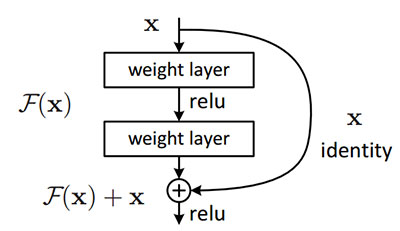
The first thing we note in the above diagram is that there is a direct link that skips several of the model's levels. The'skip connection,' as it is known, lies at the core of residual blocks. Because of the skip connection, the output is not the same. Without the skip connection, input 'X is multiplied by the layer's weights, then adding of a bias term.

The Architecture design is inspired on VGG-19 and has a 34-layer plain network to which shortcut and skip connections are added. As seen in the diagram below, these skip connections or residual blocks change the design into a residual network.

Complete Architecture:

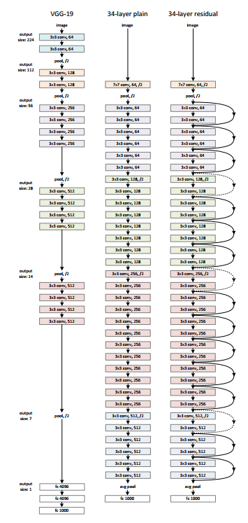
The idea was that the deeper layers shouldn't have any more training mistakes than their shallower equivalents. To put this notion into action, skip-connections were created. The creators of this network used a pre-activation variation of the residual block in which gradients can flow through the shortcut link to the earlier layers, minimising the problem of "vanishing gradients."

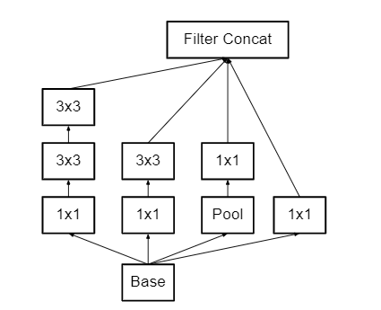
4. GoogleNet / Inception:

The ILSVRC 2014 competition was won by the GoogleNet or Inception Network, which had a top-5 error rate of 6.67 percent, which was virtually human level performance. Google created the model, which incorporates an improved implementation of the original LeNet design. This is based on the inception module concept. GoogLeNet is a variation of the Inception Network, which is a 22-layer deep convolutional neural network.

GoogLeNet is now utilised for a variety of computer vision applications, including face detection and identification, adversarial training, and so on.

The inception Module looks like this:

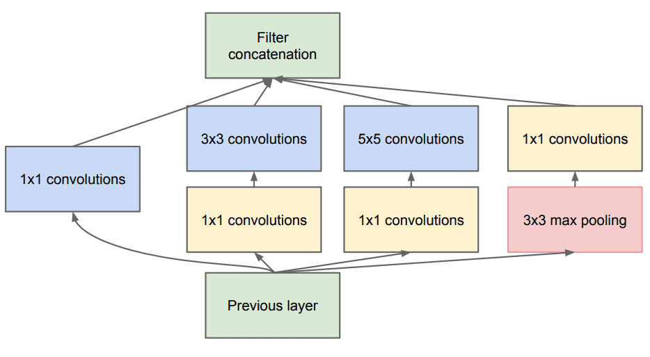
The InceptionNet/GoogleLeNet design is made up of nine inception modules stacked on top of each other, with max-pooling layers between them (to halve the spatial dimensions). It is made up of 22 layers (27 with the pooling layers). After the last inception module, it employs global average pooling.

5. MobileNetV1:

Nine inception modules are placed on top of each other in the InceptionNet/GoogleLeNet architecture, with max-pooling layers between them (to halve the spatial dimensions). There are 22 layers in all (27 with the pooling layers). It uses global average pooling after the final inception module.

The MobileNet model is built on depthwise separable convolutions, which are a type of factorised convolution that divides a regular convolution into a depthwise convolution and a pointwise convolution. The depthwise convolution used by MobileNets applies a single filter to each input channel. The depthwise convolution's outputs are then combined using an 11 convolution by the pointwise convolution. In one step, a conventional convolution filters and mixes inputs to create a new set of outputs. The depthwise separable convolution divides this into two layers: one for filtering and the other for combining.

Let’s have a look at the complete Architecture:

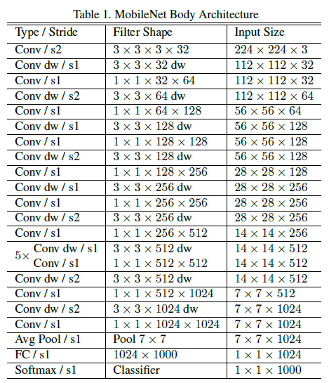
Except for the first layer, which is a complete convolution, the MobileNet structure is based on depthwise separable convolutions, as discussed in the preceding section. With the exception of the last fully connected layer, which has no nonlinearity and feeds into a softmax layer for classification, all layers are followed by a batchnorm and ReLU nonlinearity.

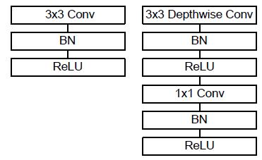
(Above Image:Standard Convolution (Left), Depthwise separable convolution (Right) With BN and ReLU)

6. ZfNet:

Zeiler and Fergus introduced a fascinating multilayer Deconvolutional NN (DeconvNet) in 2013, which became known as ZfNet (Zeiler and Fergus 2013). ZfNet was created to statistically visualise network performance. The goal of the network activity visualisation was to track CNN performance by analysing neuron activation.

It’s architecture consists of five shared convolutional layers, as well as max-pooling layers, dropout layers, and three fully connected layers. In the first layer, it employed a 77 size filter and a lower stride value. The softmax layer is the ZFNet's last layer.

7. Depth based CNNs:

Deep CNN architecture/designs are founded on the idea that as the network's depth grows, it will be able to better approximate the target function with more nonlinear mappings and enriched feature hierarchies. The success of supervised training has been attributed to the network depth.

Deep networks can express some types of function more effectively than shallow designs, according to theoretical research. In 2001, Csáji published a universal approximation theorem, which asserts that every function may be approximated with just one hidden layer. However, this comes at the expense of an exponentially large number of neurons, making it computationally non-realistic in many cases. Bengio and Delalleau proposed that deeper networks can preserve the network's expressive capability at a lower cost in this aspect.

8. Highway Networks:

Srivastava et al. presented a deep CNN called Highway Networks in 2015, based on the idea that increasing network depth can boost learning capacity. The fundamental issue with deep networks is their sluggish training and convergence times. For the effective training of deep networks, Highway Networks used depth to learn enhanced feature representation and provide a novel cross-layer connection method.

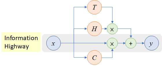
Highway Circuit

Highway Networks are also categorized as multi-path based CNN architectures. The convergence rate of highway networks with 50 layers was higher than that of thin yet deep systems. Srivastava et al. demonstrated that adding hidden units beyond 10 layers reduces the performance of a simple network. Highway Networks, on the other hand, were found to converge substantially quicker than simple networks, even at 900 layers deep.

9. Wide ResNet:

The biggest disadvantage of deep residual networks, according to some, is the feature reuse problem, in which some feature changes or blocks may contribute relatively little to learning. Wide ResNet was formed to solve this issue. The major learning potential of deep residual networks, according to Zagoruyko and Komodakis, is attributable to the residual units, whereas depth has a supplemental influence. ResNet was made wide rather than deep to take use of the residual blocks' strength.

Wide ResNet extended the network's width by adding an extra factor k, which governs the network's width. Wide ResNet shown that broadening the layers may be a more effective technique of improving performance than making residual networks deep.

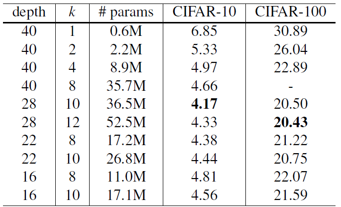
Different Width (k) and Depth on CIFAR-10 and CIFAR-100

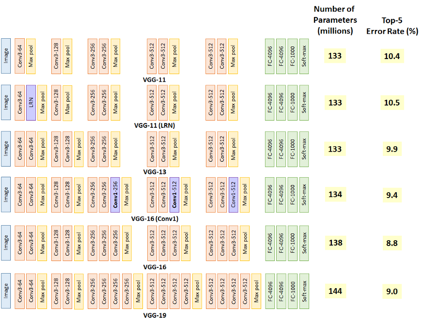
10. VGG:

VGG is a convolutional neural network design that has been around for a long time. It was based on a study on how to make such networks more dense. Small 3 x 3 filters are used in the network. The network is otherwise defined by its simplicity, with simply pooling layers and a fully linked layer as additional components.

In comparison to AlexNet and ZfNet, VGG was created with 19 layers deep to replicate the relationship between depth and network representational capability.

Small size filters can increase the performance of CNNs, according to ZfNet, a frontline network in the 2013-ILSVRC competition. Based on these observations, VGG replaced the 11x11 and 5x5 filters with a stack of 3x3 filters, demonstrating that the simultaneous placement of small size (3x3) filters may provide the effect of a big size filter (5x5 and 7x7). By lowering the number of parameters, the usage of tiny size filters gives an additional benefit of low computing complexity. These discoveries ushered in a new research trend at CNN, which is to work with lower size filters.

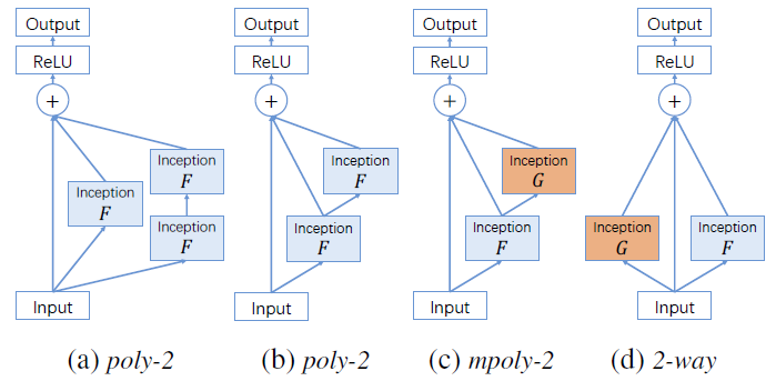
11. PolyNet:

POLYNET IS THE FIRST TOOL TO AUTOMATICALLY TRAIN AND OPTIMIZE A NEURAL NETWORK, RESULTING IN HIGHER QUALITY A.I. AND MACHINE LEARNING RESULTS.

PolyNet traverses the whole network and explores the entire space, making intelligent decisions about weights and structure so that it may automate improvements to increase performance and functionality, with better results for the end user. PolyNet is a first: a ready-to-use neural network training solution that you can implement in-house, ensuring that your data never leaves the premises. That is PolyNet's one-of-a-kind and distinguishing feature.

A PolyNet composes of polyInception module:

12. Inception v2:

The second generation of Inception convolutional neural network designs, Inception v2, employs batch normalisation.

In the architecture of Inception V2. The two 33% convolutions replace the 55% convolution. Because a 55 convolution is 2.78 more costly than a 33 convolution, this reduces computing time and hence boosts computational speed. As a result, using two 33 layers instead of 55 improves architectural performance.

nXn factorization is also converted into 1xn and nx1 factorization using this architecture. As previously stated, a 33 convolution may be reduced into 13, followed by a 31 convolution, which is 33 percent less computationally demanding than a 33 convolution.

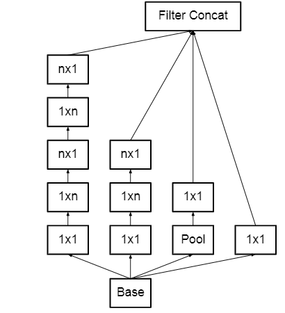
Instead of making the module deeper, the feature banks were increased to address the problem of the representational bottleneck. This would avoid the knowledge loss that occurs as we go deeper.

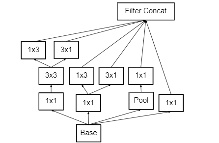
13. Inception v3 V4 and Inception-ResNet:

The upgraded versions of Inception-V1 and V2 are Inception-V3, V4, and Inception-ResNet. Inception-V3 was created with the goal of lowering the computational cost of deep networks without sacrificing generalisation. For this, Szegedy et al. employed 1x1 convolution as a bottleneck before the big filters, replacing large size filters (5x5 and 7x7) with tiny and asymmetric filters (1x7 and 1x5). When 1x1 convolution is combined with a large size filter, the standard convolution process resembles a cross-channel correlation. Lin et al. used the possibility of 1x1 filters in NIN design in one of their prior efforts. Szegedy and colleagues cleverly applied the same principle.

Inception-V3 employs a 1x1 convolutional operation, which divides the input data into three or four smaller 3D spaces, and then maps all correlations in these smaller 3D spaces using standard (3x3 or 5x5) convolutions. Szegedy et al. merged the power of residual learning with inception block in Inception-ResNet. The residual connection took the role of filter concatenation in this way.

Szegedy et al. have shown that Inception-V4 with residual connections (Inception-ResNet) has the same generalisation capacity as plain InceptionV4, but with more depth and width. They did notice, however, that Inception-ResNet converges faster than Inception-V4, indicating that training Inception networks with residual connections speeds up the process dramatically.

14. DenseNet:

DenseNet was proposed to overcome the vanishing gradient problem in the same manner as Highway Networks and ResNet were (Srivastava et al. 2015a; He et al. 2015a; Huang et al. 2017). Because ResNet expressly retains information through additive identity transformations, many layers may provide very little or no information. DenseNet uses cross-layer connection, although in a modified form, to solve this problem. In a feed-forward approach, DenseNet connects each preceding layer to the next coming layer.

As stated in equation, feature-maps from all previous levels were used as inputs into all future layers.

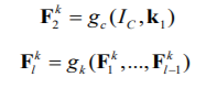
DenseNet has a thin layer structure, but as the number of feature-maps grows, it gets more parametrically costly. By giving each layer direct access to the gradients via the loss function, the network's information flow improves. On tasks with fewer training sets, direct admission to gradient contains a regularising impact, which lowers overfitting.

15. Pyramidal Net:

The depth of feature-maps rises in following layers in older deep CNN designs such as AlexNet, VGG, and ResNet due to the deep stacking of several convolutional layers. However, when each convolutional layer or block is followed by a subsampling layer, the spatial dimension diminishes. As a result, Han et al. claimed that deep CNNs' learning potential is limited by a significant rise in feature-map depth while simultaneously losing spatial information.

Han et al. suggested the Pyramidal Net to improve ResNet's learning capabilities (Han et al. 2017). In contrast to ResNet's abrupt fall in spatial breadth as depth increases, Pyramidal Net steadily increases the width per residual unit. Instead of retaining the same spatial dimension inside each residual block until down-sampling, this method allows pyramidal Net to cover all feasible places. It was given the term pyramidal Net because of the top-down steady growth in the depth of the characteristics map.

Pyramidal Net widens the network using two alternative ways, including addition and multiplication-based widening. The distinction between the two forms of widening is that the additive pyramidal structure grows linearly while the multiplicative pyramidal structure grows geometrically. However, a key drawback of the Pyramidal Net is that as the breadth grows, there is a quadratic rise in both space and time.

16. Xception:

Xception is an extreme Inception architecture that makes use of the concept of depthwise separable convolution. To control computational complexity, Xception made the original inception block bigger and replaced the multiple spatial dimensions (1x1, 5x5, 3x3) with a single dimension (3x3) followed by a 1x1 convolution. By separating spatial and feature-map (channel) correlation, Xception makes the network more computationally efficient.

Below figure depicts the Xception block's architecture:

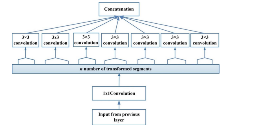
Xception simplifies computation by individually convolving each feature-map across spatial axes, then performing crosschannel correlation via pointwise convolution (1x1 convolutions). Xception's transformation technique does not lower the amount of parameters, but it does make learning more efficient and leads to better performance. Xception's transformation technique does not lower the amount of parameters, but it does make learning more efficient and leads to better performance.

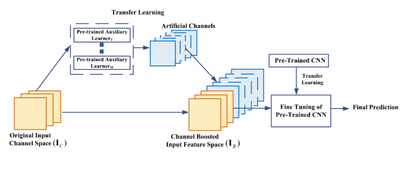
17. Channel Boosted CNN using TL:

Khan et al. developed a novel CNN architecture called Channel boosted CNN (CBCNN) in 2018 that is based on the notion of increasing the number of input channels to improve the network's representational capacity.

Channel boosting is accomplished by using auxiliary deep generative models to create additional channels, which are subsequently exploited by deep discriminative models.

The generative learners in CB-CNN are AEs, which are used to learn explanatory reasons of variation underlying the data. By supplementing the learnt distribution of the input data with the original channel space, the notion of inductive TL is applied in an unique way to generate a boosted input representation. Channel-boosting phase is encoded in a generic block that is added at the start of a deep network by CB-CNN. TL can be utilised at both the generation and discrimination stages, according to CB-CNN. The study's relevance is that it employs multi-deep learners, with generative learning models serving as auxiliary learners. These improve the deep CNN-based discriminator's representational capacity.

Below is the architecture:

18. Residual Attention Neural Network:

To enhance the network's feature representation, Wang et al. suggested a Residual Attention Network (RAN). The goal of incorporating attention into CNN was to create a network that could learn object-aware characteristics. RAN is a feed-forward CNN developed by stacking residual blocks and using the attention module. The trunk and mask branches of the attention module follow a bottom-up, top-down learning method.

Fast feedforward processing and top-down attention feedback are combined in a single feed-forward process thanks to the integration of two separate learning algorithms into the attention module. Low-resolution feature-maps with substantial semantic information are produced using a bottom-up feed-forward framework. Top-down architecture, on the other hand, generates dense characteristics in order to infer each pixel.

By stacking numerous attention modules, RAN was made efficient in recognising crowded, complicated, and noisy pictures. The capacity to adaptively allocate weight to each feature-map depending on their importance in the layers was enabled by the hierarchical architecture of RAN.

19. Attention Based CNNS:

Different degrees of abstraction play a key role in determining the NN's discriminating capacity. In addition to learning numerous hierarchies of abstractions, concentrating on context-relevant characteristics is important for picture identification and localisation. This effect is known as attention in the human visual system. Humans look at the sight in fragments and pay attention to bits that are significant to the context. This method not only assists to concentrate targeted regions, but it also deduces several interpretations of things present at that spot, assisting in the better capture of visual structure.

RNN and LSTM both have interpretability that is similar in several ways. For the creation of sequential data, RNN and LSTM networks use attention modules, and the new samples are weighted depending on their presence in prior rounds. Various scholars used the idea of attention into CNN to improve representation and overcome computational limitations. This concept of attention also aids CNN's ability to distinguish things despite busy backdrops and complicated settings.

20. Feature-Map (ChannelFMap) Exploitation based CNNs:

Because of its hierarchical learning and automated feature extraction capabilities, CNN has become useful for MV tasks. The performance of classification, segmentation, and detection modules is heavily influenced by feature selection. The weights associated with a kernel, also called as mask, are tuned in CNN to choose features dynamically. Additionally, numerous phases of feature extraction are performed, allowing for the extraction of a wide range of features (called as feature-maps or channels in CNN). Some of the feature-maps, on the other hand, play little or no function in object classification.

Large feature sets may produce a noise effect, resulting in over-fitting of the network. This implies that, in addition to network engineering, feature-map selection can have a significant impact on network generalisation. In this section, the terms feature-maps and channels will be used interchangeably because many academics refer to feature-maps as channels.

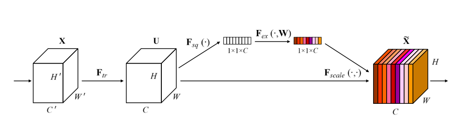
21. Squeeze and Excitation Network:

Squeeze-and-Excitation Networks, bring in a building block for Convolutional Neural Networks (CNN) that increase channel interdependencies at nearly no cost of computation.Basically Squeeze-and-excitation blocks, are an architectural element that may be placed into a convolutional neural network to boost performance while only increasing the overall number of parameters by a minimal amount

The main idea behind Squeeze-and-Excitation Networks:

Is to add parameters to every convolutional block's channel so that the network could modify the weight of every feature map adaptively.

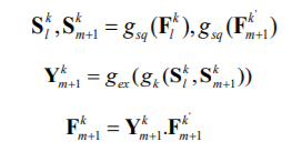
22. Competitive Squeeze and Excitation Networks

Hu et al. suggested the Competitive Inner-Imaging Squeeze and Excitation for Residual Network (CMPESE Network) in 2018. To improve the learning of deep residual networks, Hu et al. employed the SEblock concept. The feature-maps are re-calibrated by SE-Network depending on their contribution to class discrimination. The fundamental issue with SE-Net is that with ResNet, the residual information is only used to determine the weight of each feature-map. This reduces the impact of SEblock and eliminates the need for ResNet data. Hu et al. tackled the issue by creating feature-map wise motifs (statistics) from both residual and identity mapping feature-maps.

The mathematical expression for CMPE-SE block is represented using the following equation:

With this article at OpenGenus, you must have the complete idea of Different types of CNN models.