Dynamic programming for Code generation

Dynamic programming not only applies to a broad class of register machines but its application results in the generation of optimal code that runs in linear time.

Table of contents.

1. Introduction.
2. An example.
3. Code generation with dynamic programming.
4. Contiguous evaluation.
5. The algorithm.
6. Summary.
7. References.

Introduction.

We first discuss an algorithm to generate code from a labeled expression tree that works for machines whereby computations are done in registers and instructions consist of an operator that is applied to one or two registers and a memory location then proceed into the dynamic programming technique works for a broad class of register machines with a complex instruction set for which optimal code is generated in linear time.

An example - Generating code from a labeled expression tree.

Input: A labeled tree with each operand appearing once and a number of registers r ≥ 2.
Output: An optimal sequence of machine instructions to evaluate the root into a register using no more than r registers, we assume they are R1, R2, ..., Rr.
Method: We apply a recursive algorithm, starting from the root of the tree with the base b = 1 and work on each side of the trees separately then store the result in a large subtree, this is for interior nodes with label k > r.
This result is brought back from memory before node N is evaluated and the final step takes place in registers ${\mathrm{R}}_{\mathrm{r-1}}$ and ${\mathrm{R}}_{\mathrm{r}}$

The Algorithm:

1. Node N has at least one child with label r ≥ 2 therefore we pick the larger child as the big child and let the other child be little child
2. We recursively generate code for the selected big child using base b = 1 and store this result in register ${\mathrm{R}}_{\mathrm{r}}$.
3. Next, we generate the machine instruction ST${\mathrm{t}}_{\mathrm{k}}$,${\mathrm{R}}_{\mathrm{r}}$, where ${\mathrm{t}}_{\mathrm{k}}$ is a temporary variable that stores temporary results that assists in the evaluation of label k.
4. Now to generate code for the little child, if it has a label r or greater, pick base = 1, if the label of the child is j < r, pick b = r - j and recursively apply this algorithm to the little child, the result will appear in ${\mathrm{R}}_{\mathrm{r}}$
5. Generate the instruction LD ${\mathrm{R}}_{\mathrm{r-1}}$, ${\mathrm{t}}_{\mathrm{k}}$
6. If the big child is the right child of N, generate the instruction OP ${\mathrm{R}}_{\mathrm{r}}$, ${\mathrm{R}}_{\mathrm{r}}$, ${\mathrm{R}}_{\mathrm{r-1}}$. If the big child is left child generate OP ${\mathrm{R}}_{\mathrm{r}}$, ${\mathrm{R}}_{\mathrm{r-1}}$, ${\mathrm{R}}_{\mathrm{r}}$.

Code generation with Dynamic programming.

The above algorithm produces optimal code from an expression tree using time which is a linear function of the size of the tree.

This works for machines whereby all computations are done in registers whereby instructions consist of operators applied in two registers or a register and memory location.

A dynamic programming algorithm is used to extend the class of machines for which optimal code can be generated from expressions trees in linear time. This algorithm works for a broad class of register machines with complex instruction sets.

Such an algorithm is used to generate code for machines with r interchangeable registers R0, R1, ..., ${\mathrm{R}}_{\mathrm{r-1}}$ and load, store and operation instructions.

Throughout this article, we will assume that every instruction has a cost of one unit however a dynamic programming algorithm works even with instructions having their own costs.

Contiguous evaluation.

The algorithm divides the problem of generating optimal code for an expression into subproblems of generating optimal code for subexpressions of the given expression.
For example consider an expression E in the form of ${\mathrm{E}}_{\mathrm{1}}$ + ${\mathrm{E}}_{\mathrm{2}}$.
To obtain an optimal program of E, we combine optimal programs for ${\mathrm{E}}_{\mathrm{1}}$ and ${\mathrm{E}}_{\mathrm{2}}$ followed by the code to evaluate the + operator.
Subproblems for generating code for ${\mathrm{E}}_{\mathrm{1}}$ and ${\mathrm{E}}_{\mathrm{2}}$ are also solved in a similar manner.

The program produced by the dynamic programming algorithm has the following property, it evaluates expression E = ${\mathrm{E}}_{\mathrm{1}}$ op ${\mathrm{E}}_{\mathrm{2}}$ "contiguously".

Let's look at the syntax tree T for E to have a better idea:

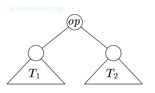
${\mathrm{T}}_{\mathrm{1}}$ and ${\mathrm{T}}_{\mathrm{2}}$ are trees for ${\mathrm{E}}_{\mathrm{1}}$ and ${\mathrm{E}}_{\mathrm{2}}$ respectively.

We say that a program P evaluates tree T contiguously if it first, evaluates the subtrees of T that need to be computed in memory followed by evaluating the remainder of T by using previously computed values from memory.

Let's look at an example of a noncontiguous evaluation:
P first evaluates part of ${\mathrm{T}}_{\mathrm{1}}$ leaving the value in a register, next it evaluates ${\mathrm{T}}_{\mathrm{2}}$ then it returns to evaluate T1.

For the register machine in this article, we prove that for any given machine-language program P that evaluates an expression tree T, there is an equivalent program P' such that;

1. It's cost is less than that of P.
2. It uses fewer registers than P.
3. P' evaluates the tree contiguously.

The above implies that every expression tree can be evaluated optimally by a contiguous program.
The contiguous evaluation property defined here above ensures for any expression tree T, there exists an optimal program consisting of optimal programs for subtrees of the root followed by an instruction to evaluate the root.
Such a property will allow us to use a dynamic programming algorithm to generate an optimal program for T.

The algorithm.

The algorithm has three phases, we assume the machine has three registers;

1. First we compute bottom-up for each node n of the expression tree T an array C of costs whereby its ith component C[i] is the optimal cost of computing the subtree S rooted at n into a register, assuming i registers are available for the computation for 1 ≤ i ≤ r.
2. Traverse T using the cost vectors to determine subtrees of T that must be computed into memory.
3. Traverse each tree using the cost vectors and associate instructions to generate the target code. The code for the subtrees that are computed into memory locations is generated first.

Each phase is implemented to run in time linearly proportional to the size of the tree.
The cost of computing a node n includes loads and stores used to evaluate S in the given number of registers and the cost of computing the operator at the root of S.
The 0th component of the cost vector is the optimal cost of computing the subtree S into memory.
The contiguous evaluation property ensures that an optimal program for S is generated by considering combinations of optimal programs only for subtrees of the root of S.
This restriction reduces the number of cases that need to be considered.

To compute the costs C[i] at node n, we look at the instructions as tree rewriting rules.
Now we consider each template E matching the input tree at node n and by examining the cost vectors at the corresponding descendants of n we determine the cost of evaluating the operands at the leaves of E.
For those operands, we consider all possible orders in which the corresponding subtrees of T can be evaluated into registers.
For each ordering, the first subtree that corresponds to a register operand is evaluated using i available registers, the second is evaluated using i-1 registers, and so on.
To account for node n, we add the cost of the instruction associated with template E.

As mentioned previously, the cost vectors for the whole tree are computed bottom-up in time linearly proportional to the number of nodes in T.
It is therefore convenient to store the instruction used to achieve the best cost for C[i] for each i at each node.
The smallest cost in the vector for the root of T yields the minimum cost of evaluating T.

An example:
We have a machine with two registers R0 and R1 and the following instructions each of unit cost.

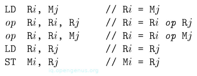
In the instructions Ri is either R0 or R1 and Mj is a memory location.
op represents any arithmetic operator.

We also have the following syntax tree.

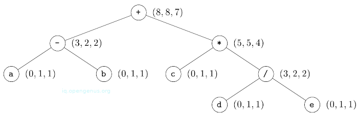
Now we apply a dynamic programming algorithm to generate optimal code for the above tree.

The first phase involves computing the cost vectors at each node.
We illustrate this cost computation by considering the cost vector at leaf a.
C[0], is the cost of computing a into memory, its value is 0 since it is already there.
C[1] is the cost of computing a into a register, its value is 1 since we can load it into a register with the instruction ld Ro, a.
C[2] is the cost of loading a into a register with two registers available, it is similar to the one with a single available register.
The cost vector at leaf a is (0, 1, 1) as can be seen from the tree.

Now we consider the cost vector at the root. First, we determine the minimum cost of computing the root with one and two registers available.
The instructions ADD RO, RO, M match the root since it is labeled with the + operator.
Using this instruction, the minimum cost of evaluating the root with a single register is the minimum cost of computing its right subtree into memory plus the minimum cost of computing its left subtree into the register plus 1 for the instruction itself.
The cost vectors at the left and right children of the root show that the minimum cost of computing the root with one register available is 5 + 2 + 1 = 8.

Looking at the minimum cost of evaluating the root with two registers available, we have three cases depending on the instructions used to compute the root and the order in which the left and right subtrees are evaluated.

The first case is to compute the left subtree with two registers available into register RO, compute the right subtree with one register available into register R1 the use the instructions ADD RO, RO, RO to compute the root. The cost is 2 + 5 + 1 = 8.

The second case is to compute the right subtree with two registers available into R1, compute the left subtree with a single register available into RO the use the instruction ADD RO, RO, RO. The cost is 4 + 2 + 1 = 7.

The third case is to compute the right subtree into a memory location M, compute the left subtree with two registers into register RO and use the instruction ADD RO, RO, M. This has a cost of 5 + 2 + 1 = 8.

The minimum cost of computing the root into memory is determined by adding 1 to the minimum cost of computing the root with all registers available, i.e, we compute the root into a register then store the result. The cost vector is at the root is (8, 8, 7).

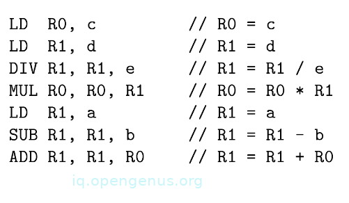
From the cost vector, we construct the code sequence by traversing the tree and we have the following optimal code sequence.

Summary.

Code generation is the final phase of a compiler .

DP has been used in various compilers e.g PCC2, its techniques facilitate re-targeting since its applicable to a broad class of machines.
A re-targetable compiler can generate code for multiple instruction sets.