
Get this book -> Problems on Array: For Interviews and Competitive Programming
In this article, we will explain the process of Fingerprint Classification and Identification using Deep Learning algorithm. It is a method of authenticating someone's identity. No two individual has the same fingerprint. The recognition system compares a fingerprint with others stored on a database to find a match or create a new identity.
Introduction
For this project, we will be using an existing code from GitHub to explain the process. The machine learning libraries used for this code,
- numpy
- keras
- matplotlib
- sklearn
- imgaug
The fingerprint dataset is downloaded from Kaggle. Sokoto Coventry Fingerprint Dataset(SOCOFing) has fingerprint images of 600 African subjects. It contains labels for gender, hand, finger names and three different altered versions. The real data were altered in these three categories; easy, medium, and hard.
The Procedure
Every deep learning projects need to follow certain steps. The algorithms can be different for each project but the approach is the same.
- A dataset of the project must be collected from online or through offline surveys.
- The dataset needs to be prepared for training, which is called preprocessing. In this process, the raw data is transformed so that it becomes suitable for the machine learning model.
- Then the dataset is divided into two groups. One is for training the model and another is for testing its accuracy.
- The final step is, applying an algorithm to train the model.
Preprocessing
Importing Libraries
As we already have our dataset, we can start preprocessing it. For that, first we will need to import some libraries that will be used for this step and throughout the whole project.
import cv2
import matplotlib.pyplot as plt
import numpy as np

import glob, os
OpenCV is used for processing the images, matplotlib is used for creating a figure, numpy is used for processing arrays, glob returns an array of filenames matching a specific pattern, and os is used for accessing a directory.
Extract Labels From Images
In this section, we will define two functions to extract the labels which are; gender, left or right hand, and finger names. These two functions are defined for two types of data, real data and altered data. They both perform the same action.
def extract_label(img_path):
    filename, _ = os.path.splitext(os.path.basename(img_path))

    subject_id, etc = filename.split('__')
    gender, lr, finger, _ = etc.split('_')

    gender = 0 if gender == 'M' else 1
    lr = 0 if lr =='Left' else 1

    if finger == 'thumb':
        finger = 0
    elif finger == 'index':
        finger = 1
    elif finger == 'middle':
        finger = 2
    elif finger == 'ring':
        finger = 3
    elif finger == 'little':
        finger = 4

    return np.array([subject_id, gender, lr, finger], dtype=np.uint16)

def extract_label2(img_path):
    filename, _ = os.path.splitext(os.path.basename(img_path))

    subject_id, etc = filename.split('__')
    gender, lr, finger, _, _ = etc.split('_')

    gender = 0 if gender == 'M' else 1
    lr = 0 if lr =='Left' else 1

    if finger == 'thumb':
        finger = 0
    elif finger == 'index':
        finger = 1
    elif finger == 'middle':
        finger = 2
    elif finger == 'ring':
        finger = 3
    elif finger == 'little':
        finger = 4

    return np.array([subject_id, gender, lr, finger], dtype=np.uint16)
These functions are splitting the texts to assign the values of the labels so that it becomes easier for the machine to process. After sorting out these data, the functions return a numpy array that contains information on every subject's gender, left or right hand, and finger names.
Real Data
A sorted list of the Real Images are stored in img_list. Then we define two numpy arrays for the images and the labels.
img_list = sorted(glob.glob('Real/*.BMP'))
imgs = np.empty((len(img_list), 96, 96), dtype=np.uint8)
labels = np.empty((len(img_list), 4), dtype=np.uint16)
for i, img_path in enumerate(img_list):
img = cv2.imread(img_path, cv2.IMREAD_GRAYSCALE)
img = cv2.resize(img, (96, 96))
imgs[i] = img
# subject_id, gender, lr, finger
labels[i] = extract_label(img_path)
np.save('dataset/x_real.npy', imgs)
np.save('dataset/y_real.npy', labels)
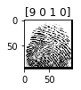
plt.figure(figsize=(1, 1))
plt.title(labels[-1])
plt.imshow(imgs[-1], cmap='gray')
In the for loop, we iterate through the image list to store the images and the labels. We use the first label extract function for Real Data. We store the images and labels in two dataset format. Using matplotlib, we can see the last image of the list.
Figure of Real:

Altered Data
The altered data has three categories. The process is the exact same as the real data but it is repeated separately for these categories. We use the second extract label function for all of the altered data.
Easy:
img_list = sorted(glob.glob('Altered/Altered-Easy/*.BMP'))
imgs = np.empty((len(img_list), 96, 96), dtype=np.uint8)
labels = np.empty((len(img_list), 4), dtype=np.uint16)
for i, img_path in enumerate(img_list):
img = cv2.imread(img_path, cv2.IMREAD_GRAYSCALE)
img = cv2.resize(img, (96, 96))
imgs[i] = img
# subject_id, gender, lr, finger
labels[i] = extract_label2(img_path)
np.save('dataset/x_easy.npy', imgs)
np.save('dataset/y_easy.npy', labels)
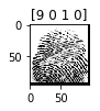
plt.figure(figsize=(1, 1))
plt.title(labels[-1])
plt.imshow(imgs[-1], cmap='gray')
Figure of Easy:

Medium:
img_list = sorted(glob.glob('Altered/Altered-Medium/*.BMP'))

imgs = np.empty((len(img_list), 96, 96), dtype=np.uint8)
labels = np.empty((len(img_list), 4), dtype=np.uint16)

for i, img_path in enumerate(img_list):
    img = cv2.imread(img_path, cv2.IMREAD_GRAYSCALE)
    img = cv2.resize(img, (96, 96))
    imgs[i] = img

    # subject_id, gender, lr, finger
    labels[i] = extract_label2(img_path)

np.save('dataset/x_medium.npy', imgs)
np.save('dataset/y_medium.npy', labels)

plt.figure(figsize=(1, 1))
plt.title(labels[-1])
plt.imshow(imgs[-1], cmap='gray')
Figure of Medium:
Hard:
img_list = sorted(glob.glob('Altered/Altered-Hard/*.BMP'))

imgs = np.empty((len(img_list), 96, 96), dtype=np.uint8)
labels = np.empty((len(img_list), 4), dtype=np.uint16)

for i, img_path in enumerate(img_list):
    img = cv2.imread(img_path, cv2.IMREAD_GRAYSCALE)
    img = cv2.resize(img, (96, 96))
    imgs[i] = img

    # subject_id, gender, lr, finger
    labels[i] = extract_label2(img_path)

np.save('dataset/x_hard.npy', imgs)
np.save('dataset/y_hard.npy', labels)

plt.figure(figsize=(1, 1))
plt.title(labels[-1])
plt.imshow(imgs[-1], cmap='gray')
Figure of Hard:
Train & Test
After the preprocessing, the dataset needs to be divided into a training set and a test set. The training data will be fed to the model to be prepared and the test data will be used for testing how well the model works.
Import Libraries
For this part, we need to import some more libraries.
import keras
from keras import layers
from keras.models import Model
from sklearn.utils import shuffle
from sklearn.model_selection import train_test_split
from imgaug import augmenters as iaa

import random
We are using Tensorflow backend for this project. sklearn and keras provides some very useful methods for deep learning models. Augmentation is used for transforming images in new and better versions.
Loading and Splitting Datasets
Loading
Loading the preprocessed datasets that we previously saved.
x_real = np.load('dataset/x_real.npz')['data']
y_real = np.load('dataset/y_real.npy')
x_easy = np.load('dataset/x_easy.npz')['data']
y_easy = np.load('dataset/y_easy.npy')
x_medium = np.load('dataset/x_medium.npz')['data']
y_medium = np.load('dataset/y_medium.npy')
x_hard = np.load('dataset/x_hard.npz')['data']
y_hard = np.load('dataset/y_hard.npy')
Images are stored in x values and labels are in y values. We are using the load function of numpy for these datasets.
Splitting
Before dividing into two groups, we unite the three categories of altered data. Only the altered data is being split into two groups.
x_data = np.concatenate([x_easy, x_medium, x_hard], axis=0)
label_data = np.concatenate([y_easy, y_medium, y_hard], axis=0)

x_train, x_val, label_train, label_val = train_test_split(x_data, label_data, test_size=0.1)
A numpy function unites the three categories and train_test_split method divides the data. the test_size determines the proportion of data falls into the test set.
Creating Complete Train-Test Set
In this section, we create sets of both real and altered data for the model. To store the labels of real data, we create a dictionary as a lookup table.
label_real_dict = {}

for i, y in enumerate(y_real):
    key = y.astype(str)
    key = ''.join(key).zfill(6)

    label_real_dict[key] = i
We create a class to generate data for the combined train and test sets. This class accepts the data, batch size and creates the set.
class DataGenerator(keras.utils.Sequence):
    def __init__(self, x, label, x_real, label_real_dict, batch_size=32, shuffle=True):
        'Initialization'
        self.x = x
        self.label = label
        self.x_real = x_real
        self.label_real_dict = label_real_dict

        self.batch_size = batch_size
        self.shuffle = shuffle
        self.on_epoch_end()

    def __len__(self):
        #Denotes the number of batches per epoch
        return int(np.floor(len(self.x) / self.batch_size))
This class returns the number of batches will be trained each time. Now we generate the batches.
    def __getitem__(self, index):
        #Generate one batch of data
        # Generate indexes of the batch
        x1_batch = self.x[index*self.batch_size:(index+1)*self.batch_size]
        label_batch = self.label[index*self.batch_size:(index+1)*self.batch_size]

        x2_batch = np.empty((self.batch_size, 90, 90, 1), dtype=np.float32)
        y_batch = np.zeros((self.batch_size, 1), dtype=np.float32)

        # augmentation
        if self.shuffle:
            seq = iaa.Sequential([
                iaa.GaussianBlur(sigma=(0, 0.5)),
                iaa.Affine(
                    scale={"x": (0.9, 1.1), "y": (0.9, 1.1)},
                    translate_percent={"x": (-0.1, 0.1), "y": (-0.1, 0.1)},
                    rotate=(-30, 30),
                    order=[0, 1],
                    cval=255
                )
            ], random_order=True)

            x1_batch = seq.augment_images(x1_batch)

        # pick matched images(label 1.0) and unmatched images(label 0.0) and put together in batch
        # matched images must be all same
        for i, l in enumerate(label_batch):
            match_key = l.astype(str)
            match_key = ''.join(match_key).zfill(6)

            if random.random() > 0.5:
                # put matched image
                x2_batch[i] = self.x_real[self.label_real_dict[match_key]]
                y_batch[i] = 1.
            else:
                # put unmatched image
                while True:
                    unmatch_key, unmatch_idx = random.choice(list(self.label_real_dict.items()))

                    if unmatch_key != match_key:
                        break

                x2_batch[i] = self.x_real[unmatch_idx]
                y_batch[i] = 0.

        return [x1_batch.astype(np.float32) / 255., x2_batch.astype(np.float32) / 255.], y_batch

    def on_epoch_end(self):
        if self.shuffle == True:
            self.x, self.label = shuffle(self.x, self.label)
We create one batch of data with the altered version and two numpy arrays for the real data. Then we augment the altered images.
The real data is compared to see if it already exists in the lookup table. It it isn't, then it is enlisted to the list and a mutual label batch is generated. This function returns the combined image batch array and a label batch.
These values are stored in two variables that will be used as train and test set.
train_gen = DataGenerator(x_train, label_train, x_real, label_real_dict, shuffle=True)
val_gen = DataGenerator(x_val, label_val, x_real, label_real_dict, shuffle=False)
Model Creation and Training
For creating and training the model, we are using Neural Network algorithm. So, we are creating multiple layers for processing the data. We maintain the exact shape for the inputs and outputs.
Conv2D layer is used for adjusting the image and MaxPooling2D is used for highlighting the features of the image. The activation function decides whether a neuron should be activated or not.
Rectified linear unit (ReLU) is the most widely used activation function as it does not activate all the neurons at the same time. We create a featur_model by specifying the input and output layers.
x1 = layers.Input(shape=(90, 90, 1))
x2 = layers.Input(shape=(90, 90, 1))
# share weights both inputs
inputs = layers.Input(shape=(90, 90, 1))
feature = layers.Conv2D(32, kernel_size=3, padding='same', activation='relu')(inputs)
feature = layers.MaxPooling2D(pool_size=2)(feature)
feature = layers.Conv2D(32, kernel_size=3, padding='same', activation='relu')(feature)
feature = layers.MaxPooling2D(pool_size=2)(feature)
feature_model = Model(inputs=inputs, outputs=feature)
# 2 feature models that sharing weights
x1_net = feature_model(x1)
x2_net = feature_model(x2)
# subtract features
net = layers.Subtract()([x1_net, x2_net])
net = layers.Conv2D(32, kernel_size=3, padding='same', activation='relu')(net)
net = layers.MaxPooling2D(pool_size=2)(net)
net = layers.Flatten()(net)
net = layers.Dense(64, activation='relu')(net)
net = layers.Dense(1, activation='sigmoid')(net)
model = Model(inputs=[x1, x2], outputs=net)
model.compile(loss='binary_crossentropy', optimizer='adam', metrics=['acc'])
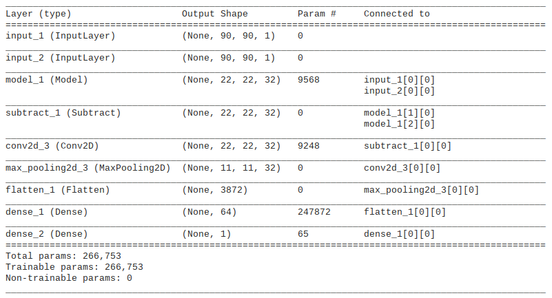
model.summary()
The subtract layer takes two inputs which are outputs of the feature_model and returns a single input while maintaining the same shape. This is used for the input layer of our actual model.
Then we flatten the input and create the output layers for the model. The Dense layer contains the connected neurons where every neuron takes the input from the neurons of the previous layer.
After creating the model, we compile to see the accuracy of its performance. The summary of the model is,
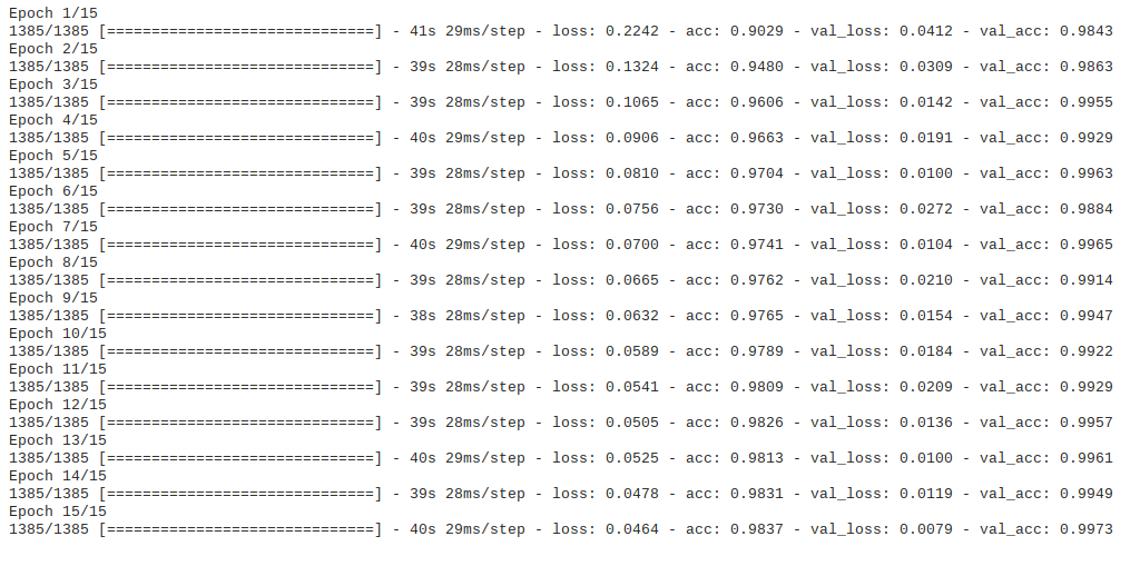
Now we train the model and examine the accuracy for 15 epochs.
history = model.fit_generator(train_gen, epochs=15, validation_data=val_gen)
Evaluate The Model
We can test to see if the model can make predictions on user input fingerprints.
We assign random index for the image and its label based on the value of altered training images. Then we augment the image for transforming it into a better version.
# new user fingerprint input
random_idx = random.randint(0, len(x_val))

random_img = x_val[random_idx]
random_label = label_val[random_idx]

seq = iaa.Sequential([
    iaa.GaussianBlur(sigma=(0, 0.5)),
    iaa.Affine(
        scale={"x": (0.9, 1.1), "y": (0.9, 1.1)},
        translate_percent={"x": (-0.1, 0.1), "y": (-0.1, 0.1)},
        rotate=(-30, 30),
        order=[0, 1],
        cval=255
    )
], random_order=True)

random_img = seq.augment_image(random_img).reshape((1, 90, 90, 1)).astype(np.float32) / 255.
We compare this random image to the real data to find a match or unmatch and make predictions on both.
# matched image
match_key = random_label.astype(str)
match_key = ''.join(match_key).zfill(6)

rx = x_real[label_real_dict[match_key]].reshape((1, 90, 90, 1)).astype(np.float32) / 255.
ry = y_real[label_real_dict[match_key]]

pred_rx = model.predict([random_img, rx])

# unmatched image
unmatch_key, unmatch_idx = random.choice(list(label_real_dict.items()))

ux = x_real[unmatch_idx].reshape((1, 90, 90, 1)).astype(np.float32) / 255.
uy = y_real[unmatch_idx]

pred_ux = model.predict([random_img, ux])

plt.figure(figsize=(8, 4))
plt.subplot(1, 3, 1)
plt.title('Input: %s' %random_label)
plt.imshow(random_img.squeeze(), cmap='gray')
plt.subplot(1, 3, 2)
plt.title('O: %.02f, %s' % (pred_rx, ry))
plt.imshow(rx.squeeze(), cmap='gray')
plt.subplot(1, 3, 3)
plt.title('X: %.02f, %s' % (pred_ux, uy))
plt.imshow(ux.squeeze(), cmap='gray')
Plotting the random image and the predictions, we can see:
Random Image, Match Image, Unmatch Image
