Pneumonia Detection on Chest X-Rays with Deep Learning [DL Project]

In this article, we have developed a Deep Learning model to detect Pneumonia from Chest X-Rays and get a performance similar to a Radiologist. This is a good project for Deep Learning Engineer Portfolio.

We have summarized the key points from the paper titled "CheXNet: Radiologist-Level Pneumonia Detection on Chest X-Rays with Deep Learning".

1. Introduction:

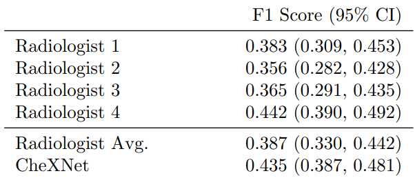
Pneumonia is an dangerous and serious disease, in US only there are more than 1 million adult who hospitalized with pneumonia and around 50000 death yearly. and one of the most efficient way to detect it is the chest X ray, however, detecting pneumonia in chest X-rays is a challenging task that relies on the availability of expert radiologists and their experience. So this paper suggest a neural network model that can give an efficient results comparing to 4 experienced radiologists that had 4, 7, 25, and 28 years of experience, not only mimic them but also exceed their average on F1 metric (which is the harmonic average of the precision and recall of the models).

2. problem statement:

• For Pneumonia detection:
  In the project our problem is to classify a frontal-view chest X-ray image X
  to (Y) either a presence of pneumonia (1) or absence of it (0) which is clearly a binary classification problem.
  So, our loss function will be binary cross entropy, but due to imbalanced data the paper suggest using weighted binary cross entropy loss function as following:
  L(X, y) = (−w+ y log p(Y = 1|X)) (−w− (1 − y) log p(Y = 0|X))
  where w+ is the weight of negative examples and w- weight of positive examples.

• For multiple thoracic pathologies:
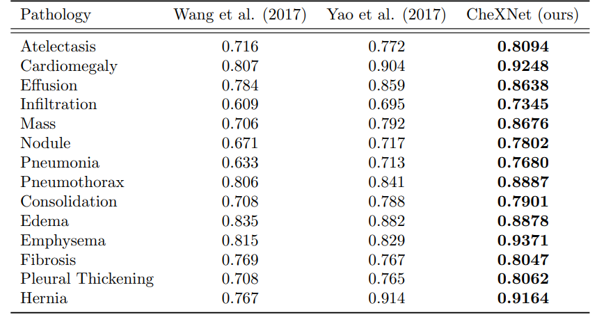
  the 14 thoracic diseases are : Atelectasis, Cardiomegaly, Consolidation, Edema, Effusion, Emphysema, Fibrosis, Hernia, Infiltration, Mass, Nodule, Pleural Thickening, Pneumonia, and Pneumothorax.**
  The paper suggest expanding the algorithm to classify the 14 diseases by :

  • instead of yielding one unit for one binary label, make the model output 14 unit for 14 binary labels indicating the presence or the absence of each disease.
  • So, the final FC layer will have 14 units instead of one.
  • And also now there is no need for weighted binary cross entropy loss, we can use the unweighted one.

2. CheXNet

Our classification problem consider a binary classification where images are classified as absence or presence of pneumonia (0 or 1 respectively) so we can use binary cross entropy loss function or the weighted one (log loss).

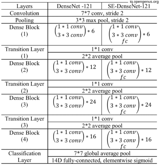
CheXNet is a 121-layer Dense Convolutional Network (DenseNet) that pretrained on image-net dataset for initial weights, then modify the last fully connected layer with a one with single unit with sigmoid non-linearity activation function. training these final model on ChestX-ray14 dataset which contains 112,120 frontal-view X-ray images of 30,805 unique patients which had different 14 labels for different 14 thoracic diseases, but we modify images labels that have pneumonia as one of the annotated pathologies as positive examples and label all other images as negative examples.(this for pneumonia detection task) OR make simple modifications to
CheXNet to detect all 14 diseases in ChestX-ray14 and leave the annotated dataset as it is.

Using Adam optimizer with standard hyper-parameters (β1 = 0.9 and β2 = 0.999), Batch size equal 16 and learning rate equal 0.001 and decayed with a factor of 10 each time the validation loss plateaus after an epoch. Then downscale the images to 224 * 224 before entering the model.

3. Dataset used:

The paper use ChestX-ray14 dataset that contain 112,120 frontal-view X-ray images of 30,805 unique patients. in the original dataset each image has a label of different 14 thoracic disease but for the pneumonia detection purposes they relabel images with pneumonia as positive or 1 and all the other images as negative or 0.

Then splitting the dataset to train/val/test split according to splitting the dataset into training (28744 patients, 98637 images), validation (1672 patients, 6351 images), and test (389 patients, 420 images). There is no patient overlap between the sets.

Then down scaling the image resolution to 224, 224 to match the model input shape also some augmentation methods like random horizontal flipping.

3. Code for model:

We can implement the model in tensorflow as follow:

For pneumonia detection model

import tensorflow as tf

input_shape = (224,224,3)
input = tf.keras.layers.Input(input_shape)
base_model=tf.keras.applications.DenseNet121(input_shape=input_shape, weights= "ImageNet", include_top=False)
x = base_model.output
x=tf.keras.layers.GlobalAveragePooling2D()(x)
x = Dense(1024, activation='relu')(x)
predictions = Dense(1, activation='sigmoid')(x)

for layer in base_model.layers:
    layer.trainable= False
model =  tf.keras.models.Model(inputs=input, outputs=prediction)

and the compiler:

import keras.backend as K
optimizer = tf.keras.optimizers.Adam(beta_1=0.9, beta_2=0.999)


def weighted_binary_crossentropy(weights):

    def w_binary_crossentropy(y_true, y_pred):
        # Calculate the binary crossentropy
        binary_crossentropy = K.binary_crossentropy(y_true, y_pred)

        # Apply the weights
        weights_tensor = y_true * weights[1] + (1. - y_true) * weights[0]
        weighted_binary_crossentropy = weights_tensor * binary_crossentropy

        return K.mean(weighted_binary_crossentropy)

    return w_binary_crossentropy
loss = weighted_binary_crossentropy([0.07,0.93])
model.compile(optimizer=optimizer, loss=loss, metrics=['accuracy'])

And For all 14 diseases detection model

import tensorflow as tf

input_shape = (224,224,3)
input = tf.keras.layers.Input(input_shape)
base_model=tf.keras.applications.DenseNet121(input_shape=input_shape, weights= "ImageNet", include_top=False)
x = base_model.output
x=tf.keras.layers.GlobalAveragePooling2D()(x)
x = Dense(1024, activation='relu')(x)
predictions = Dense(14, activation='sigmoid')(x)

for layer in base_model.layers:
    layer.trainable= False
model =  tf.keras.models.Model(inputs=input, outputs=prediction)

and the compiler:

optimizer = tf.keras.optimizers.Adam(beta_1=0.9, beta_2=0.999)
loss = tf.keras.losses.BinaryCrossentropy()
model.compile(optimizer=optimizer, loss=loss, metrics=['AUC'])

So, no of parameters depend on implementation,
Here's the breakdown of the parameters for each layer in the CheXNet model:

• Convolutional layers:
• Conv2D (7x7, 64) = 9,472
• BatchNormalization = 256
• Conv2D (1x1, 64) = 4,160
• BatchNormalization = 256
• Conv2D (3x3, 192) = 110,784
• BatchNormalization = 512
• Conv2D (1x1, 192) = 39,264
• BatchNormalization = 512
• Conv2D (3x3, 384) = 663,936
• BatchNormalization = 1,024
• Conv2D (1x1, 384) = 147,840
• BatchNormalization = 1,024
• Conv2D (3x3, 256) = 884,992
• BatchNormalization = 512
• Conv2D (1x1, 256) = 66,560
• BatchNormalization = 512
• Conv2D (3x3, 256) = 590,080
• BatchNormalization = 512
• Conv2D (1x1, 256) = 131,328
• BatchNormalization = 512
• Fully-connected layers:
• Dense (4,096) = 8,388,608
• BatchNormalization = 4,096
• Dense (4,096) = 16,781,312
• BatchNormalization = 4,096
• Dense (14) = 57,478

The total number of trainable parameters is the sum of the parameters in each layer, which is approximately 14.3 million.

4. CheXNet vs. Radiologist Performance :

The primary evaluation metric used in the CheXNet paper was the area under the receiver operating characteristic curve (AUC-ROC). However, the paper also reported the F1 score as a secondary metric.

The AUC-ROC is a common metric used in binary classification problems to evaluate the performance of a classifier, while the F1 score is a measure of a classifier's accuracy that takes into account both precision and recall.

Also the great performance of the model but the authors identified some limitations, such that only frontal radiographs were presented to the radiologists and model during diagnosis, but it has been shown that up to 15% of accurate diagnoses require the lateral view, and also the model and the experts didn't know the history of patients which in turn decrease the radiologists performance.

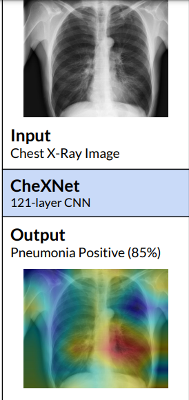
The model not only correctly classify the pathology but also highlight the areas of the X-ray that are most important for making a particular pathology classification using class activation maps(CAMs) or the Grad-CAM techniques.

.

Finally i want to thank you for reading and following the article at OpenGenus.