
Environmental perception and scene understanding are very important aspect within the field of autonomous vehicles that provides crucial information for the car to take decisions, including but not limited to detecting surrounding obstacles, identifying traffic light, and measuring distances. Semantic Segmentation is a widely known perception method that is used in self-driving cars. It partitions an image into several coherent semantically meaningful parts and classifies each part into one of the pre-determined classes.
In this article, we will choose a model and fine-tune it to segment a dataset designed for autonomous driving. This involves buildings and road segmentation.
Table of Content
- How autonomous vehicles work ?
- Dataset Description
- Create Data Pipeline
- Train your model
- Evaluation
- Comparison
- Conclusion
1. How autonomous vehicles work?
This section gives general information about autonomous vehicles, the reader is free to skip it and go to the next section, it wouldn't affect their understanding for the rest of the article. For those interested in learning more, I hope you will enjoy it.
Self-driving vehicles are made up of: sensors, actuators, machine learning systems, software and processors to execute the software.
Sensors are the main source of data for self-driving cars. There are radar sensors, video cameras,lidars (light detection and ranging) and ultrasonic sensors that are spread in different parts of the vehicle.
Radar sensors monitor the position of nearby vehicles, while video cameras capture road signs, traffic lights, pedestrians, roads and track other vehicles. Lidars bounce pulses of light to measure distances and detect edges. Lidars are optional, some companies like Tesla choose not to use them since the informations extracted from them can also be extracted from the images collected by the cameras. Finally, ultrasonic sensors are located in the wheels to detect curbs and other vehicles when parking.
The collected data will then be sent to the vehicle's computer that will execute different algorithms like object recognition/detection, obstacles avoidance and predictive modeling. As a result, a set of instructions will be sent to the actuators to navigate the car.
Note that the actuators are responsible for the car's acceleration, braking and steering.
2. Dataset Description and Exploration
The dataset used in this article is Camvid dataset more specifically CamSeq01 Dataset. It is a video sequence of high resolution images, that is designed specifically for the problem of autonomous driving.
The sequence has been recorded in a moving vehicle in the city of Cambridge. You can find the link to the dataset here.
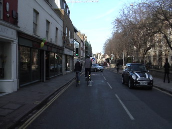
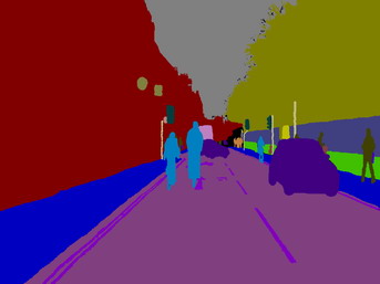
The dataset has 101 images with size 960x720 pixels. Each pixel has been manually labelled to one of 32 classes. The figure below shows an image sample from the dataset and its ground Truth map segmentation.
To explore this dataset, let's start by looking to the distribution of the 32 classes.
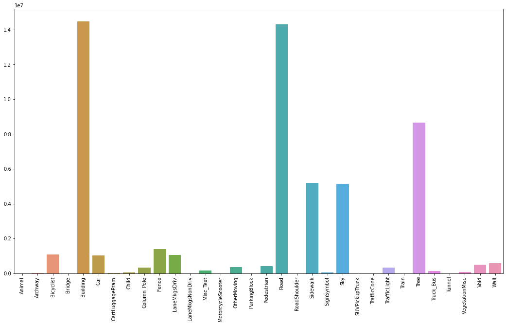
Clearly the dataset is imbalanced, which is a common problem in datasets of street scenes, where scene images have usually more roads, buildings and trees rather than pedestrians. This is problematic since it may bias the training process. To tackle the problem we will weight the classes and pass those weights to the loss function.
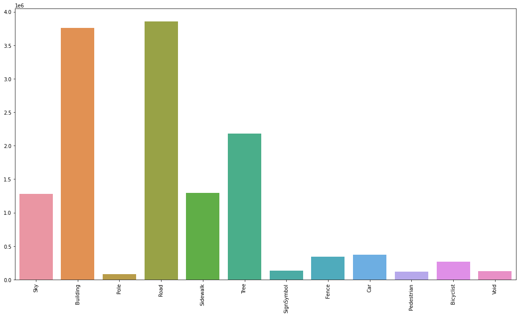
Additionally, notice that there are many classes that can be grouped together like: Car,SUVPickupTruck, Truck_Bus, Train and OtherMoving or Tree and VegetationMisc. Grouping similar classes will help in simplifying the problem to the model, rather than predicting 32 classes, it will predict only 12 classes.
Great! now that we know how our data looks like, we are now ready to prepare it for the training and the inference.
3. Create Data Pipeline
The code of this project may be found here. In the following paragraphs I will try to explain the code and help you reproduce the project.
So start by creating a virtual environment and copy the requirements.txt file.
Then install the required packages by running the following command:
pip install -r requirements.txt
Now, we need to download the dataset. So start by creating utils folder and copy inside of it the file download_dataset.py. The file has only one function that runs a wget command to download the dataset, then unzips the dataset and deletes the zip file.
Run the following command in the root directory of your project to download the dataset.
python ./utils/download_dataset.py --savedir="./dataset/camvid/"
Let's pass to creating our Data pipeline. Create a file called data.py inside a folder called data_handler. We will handle all the data processing part in this file.
We will start by overriding the class torch.Dataset to adapt it to our dataset. For this we need to override the following methods: _init_ , _len_ and _getitem_
- The init method will take in the necessary configurations for the class. We will need the parent file of the dataset, the list of paths to all the images and masks, a feature extractor to prepare and adapt the data to the model we will be sing later and a boolean to indicate whether to apply or not data augmentation to the dataset.
- len method should return the size of the dataset
- getitem function will be called when iterating through the dataset. It is responsible for preparing the images and masks, applies data augmentation on them if the augment boolean is set to true and then return the resulted image and its corresponding segmentation map (mask).
class CamvidDataset(Dataset):

  def __init__(self,
               root_dir,
               image_filenames,
               masks_filenames,
               feature_extractor,
               augment=False,
               num_classes=12) -> None:

    self.root_dir = root_dir
    self.image_filenames = image_filenames
    self.masks_filenames = masks_filenames
    self.num_classes = num_classes
    self.feature_extractor = feature_extractor


    conf_file = os.path.join(root_dir,'label_colors11.txt')

    colors, labels = self._dataset_conf(conf_file)
    self.id2label = dict(zip(range(self.num_classes),labels))
    self.class_colors = labelColors
def __len__(self):
    return len(self.image_filenames)
def __getitem__(self,idx):

    image_filename = self.image_filenames[idx]
    mask_filename = self.masks_filenames[idx]

    image = cv2.imread(os.path.join(self.root_dir,image_filename),)# BGR image
    mask = cv2.imread(
            os.path.join(self.root_dir,mask_filename),
            cv2.IMREAD_UNCHANGED,
        ) # BGR image

    # convert the mask from bgr to grayscale
    mask = self.bgr2gray12(mask,self.class_colors)

    if self.augment :
      image, mask = self._data_augmentation(image,mask)

    encod_inputs =self.feature_extractor(image,mask, return_tensors='pt')

    for k,v in encod_inputs.items():
      encod_inputs[k].squeeze_()

    return encod_inputs
To define our data augmentation pipeline, there are many open source libraries for this, like: augmentor, imgaug, albumentations, SOLT. I personally like Albumentations, I find it fast compared to others and also it has many image processing transformations. So in this article I will be using Albumentations, but feel free to use the library of your choice.
One additional note is that our dataset is composed of RGB images, so it is better to apply both position based augmentations and color based augmentations. If the images were Grayscale, position based augmentations are sufficient.
def _data_augmentation(self, image, mask):
    aug = A.Compose(
      [
          A.Flip(p=0.5),
          A.RandomRotate90(p=0.5),
          A.OneOf([
                  A.Affine(p=0.33,shear=(-5,5),rotate=(-80,90)),
                  A.ShiftScaleRotate(
                    shift_limit=0.2,
                    scale_limit=0.2,
                    rotate_limit=120,
                    #border_mode= cv2.BORDER_CONSTANT,
                    #value=255, # padding with the ignored class
                    p=0.33),
                  A.GridDistortion(p=0.33),
                ], p=1),
          A.CLAHE(p=0.8),
          A.OneOf(
              [
                  A.ColorJitter(p=0.33),
                  A.RandomBrightnessContrast(p=0.33),
                  A.RandomGamma(p=0.33)
              ],
              p=1
          )
          ]
    )
    augmentation = aug(image=image, mask=mask)
    aug_img, aug_mask = augmentation['image'], augmentation['mask']
    return aug_img, aug_mask
An idea to keep in mind is that applying a data augmentation pipeline will not add more images to the dataset, what will happen instead is that for the same image _getitem_ will apply a different transformation and thus will return a different result, tricking like this the model that there are more images.
Let's create a function to return the training and validation dataset. Notice in the code bellow, we resized the images to their half sizes, this is to prevent your code from crashing. We also did rescale the images with the default factor (1/255) to speed up the learning.
# Returns a non batched dataset
def get_dataset(data_path='/dataset/camvid/',
                val_split=0.2,
                random_state=42,
                feature_extractor_name='nvidia/segformer-b2-finetuned-cityscapes-1024-1024'):

  feature_extractor = SegformerImageProcessor.from_pretrained(feature_extractor_name)
  feature_extractor.do_reduce_labels = False
  feature_extractor.do_resize = True
  feature_extractor.size = {"height":360, "width":480}
  feature_extractor.do_normalize= False
  feature_extractor.do_rescale= True


  img_files, mask_files = get_data_filenames(data_path)

  train_imgs, val_imgs, train_masks, val_masks = train_test_split(
      img_files, mask_files, test_size=val_split, random_state=random_state, shuffle=True)

  train_dataset = CamvidDataset(data_path,
                                train_imgs, train_masks,
                                feature_extractor,
                                augment=True,
                                num_classes=12
                                )
  val_dataset = CamvidDataset(data_path,
                              val_imgs,
                              val_masks,
                              feature_extractor,
                              num_classes=12)
  return train_dataset, val_dataset
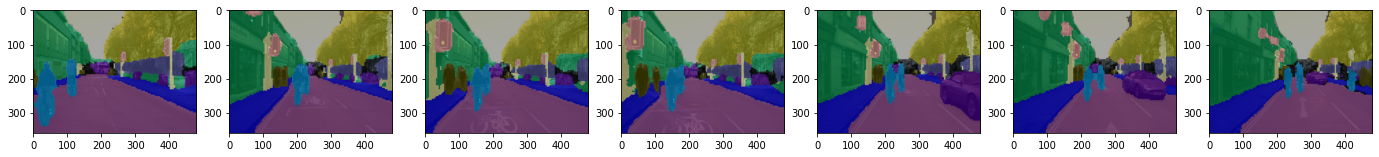
The figure bellow shows a sample of the augmented images.
We still have one problem with our data, which is class imbalance. To tackle this problem, we only need to compute the frequency inverse for each class and then later we will pass these weights to the loss function. With this approach, minority classes will have bigger weights and majority classes will have lower weights, thus the loss function will penalize more the misclassification made by minority classes and will penalize less the misclassification made by majority classes.
# counts number of samples in each class
def compute_class_distribution(dataset):
  summary = [0]*dataset.num_classes

  for inputs in dataset:
      mask = inputs['labels']
      labels, counts = np.unique(mask, return_counts=True)
      for idx,label in enumerate(labels):
        summary[label] += counts[idx]
  return summary

# computes the weight of each class
def compute_class_weights(total, class_counts):
  weights = []
  for class_count in class_counts:
    weights.append(total/class_count)
  return weights
Now that our data is ready, we need to wrap it with pytorch DataLoader class to batch the data, create an iterable and serve it to the model for training.
One of the most important parameters to pass to DataLoader are:
- num_workers: it is the number of subprocess that will be running in parallel to load the data. It is advisable that you set this parameter to a number less than the total number core CPUs you have to avoid some overheads.
- prefetch_factor: is the number of preloaded batches while the GPU is performing the computation. Meaning if you set num_workers to 2 and prefetch_factor to 2, the daraloader will prepare 2*2=4 batches of data. So if you don't have enough memory, take caution on lowering this parameter.
# Returns batched dataset
def get_dataloader(dataset,
                   train_batch_size=10,
                   val_batch_size=7,
                   num_workers=2,
                   prefetch_factor=5):


  train_dataset, val_dataset = dataset[0], dataset[1]

  train_dataloader = DataLoader(train_dataset,
                                batch_size=train_batch_size,
                                shuffle=True,
                                num_workers=num_workers,
                                prefetch_factor=prefetch_factor)

  val_dataloader = DataLoader(val_dataset,
                              batch_size=val_batch_size,
                              num_workers=num_workers,
                              prefetch_factor=prefetch_factor)

  return train_dataloader, val_dataloader
4. Train your model
Before choosing the correct model, it is good to keep in mind that your model is going to be used in embedded systems and for real-time processing. But what does this means?
The first point is that embedded systems have less memory and less computational power than normal computers and servers. Additionally the more time it is required by your model to make inference (prediction) the more energy it is consumed from your system leading it to overheat. Thus you want to make sure that your model is:
- Small enough to fit in the memory
- Simple enough to make good predictions while being cheaper computationally to run and thus consumes less energy.
The second point is about Real-time processing, the data flow is infinite which requires a small latency, which takes us again to the fact that your model should be computationally cheaper with good enough precision.
Great with these ideas in mind, we are looking for a model that is small and efficient. Some examples of such models are:
| Model | Number of parameters | Applicable Real-time |
|---|---|---|
| MobileNet [1] | 14M | Yes |
| MobileVit[3] | 2.3 M | Yes |
| SegFormer (B0-B2)[2] | 3 M-27.4M | Yes |
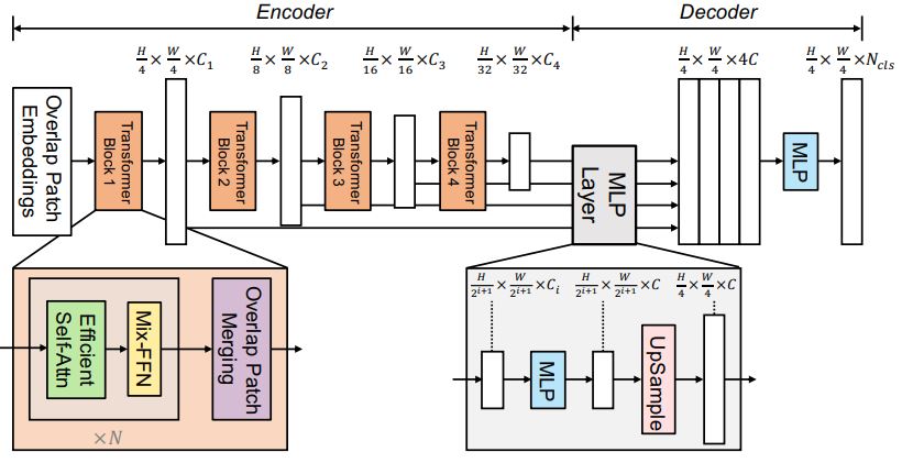
For the purpose of this article, we will be fine tuning SegFormer model from Hugging Face's library transformers.
SegFormer [2] is a transformer based model. It is composed of a hierarchical transformer encoder, that is inspired from the Vision Transformer (ViT) but optimized for the semantic segmentation task, and a lightway all-MLP decoder.
If you never heard about the vision transformer, then this article may be a good starting point, but for now you can just follow up with this tutorial.
First start by creating a file and name it model.py and place it in a folder called model_buildr. This file will allow us to create, train and load our model.
Our starting model is a pre-trained segformer on cityscapes dataset. We will wrap this model in Pytorch LightningModule class to customize the training loop. We will also use Pytorch Trainer class to train the model.
Overriding a LightningModule class requires defining the following methods:
- _init_ : to take all model's parameters and hyper-parameters
- train_step : to define the training loop
- forward: computes the predictions of the model.
- validation_step: optional
- configure_optimizers: return the optimizer used for adjusting the model's parameters.
- train_dataloader and validation_dataloader: returns the data loaders that we created at the end of the previous section.
For evaluation, we will be monitoring the mean accuracy and the mean intersection over union (mean_iou) using Eval package from Hugging Face.
Recall that in the previous section we computed the weights of each class, in the section bellow we will pass these weights to the weighted cross entropy loss used to train this model.
The outputs of segformer are 4 times smaller than the original size, thus we need to upsample the predictions to their original size before computing the loss. I used for that the nearest neighbor interpolation.
class SegFormerFineTuned(pl.LightningModule):
  def __init__(self, id2label,
               train_dl,
               val_dl,
               metrics_interval,
               class_weights,
               model_path="nvidia/segformer-b2-finetuned-cityscapes-1024-1024"):

    super(SegFormerFineTuned, self).__init__()
    self.id2label = id2label
    self.metrics_interval = metrics_interval
    self.train_dl = train_dl
    self.val_dl = val_dl
    self.weights = class_weights
    self.model_path = model_path

    self.num_classes = len(id2label.keys())
    self.label2id = {v:k for k,v in self.id2label.items()}

    self.model = SegformerForSemanticSegmentation.from_pretrained(
        self.model_path,
        return_dict=False,
        num_labels=self.num_classes,
        id2label=self.id2label,
        label2id=self.label2id,
        ignore_mismatched_sizes=True,
    )

    self.train_mean_iou = evaluate.load("mean_iou")
    self.val_mean_iou = evaluate.load("mean_iou")
    self.test_mean_iou = evaluate.load("mean_iou")

    # Save the hyper-parameters
    # with the checkpoints
    self.save_hyperparameters()

  def forward(self, images, masks):
    outputs = self.model(pixel_values=images)
    return (outputs)

  def training_step(self, batch, num_batch):
    images, masks = batch['pixel_values'], batch['labels']

    # Forward pass

    predictions = self(images,masks)[0]

    # upsample the predictions
    # from size (H/4,W/4) -> (H,W)
    predictions = torch.nn.functional.interpolate(
            predictions,
            size=masks.shape[-2:],
            mode="nearest-exact",
            align_corners=False
        )

    weighted_loss = CrossEntropyLoss(weight=self.weights,ignore_index=255)
    loss = weighted_loss(predictions,masks)

    predictions = predictions.argmax(dim=1)


    # Evaluate the model
    self.train_mean_iou.add_batch(
            predictions= predictions.detach().cpu().numpy(),
            references=masks.detach().cpu().numpy()
        )
    if num_batch % self.metrics_interval == 0:

        metrics = self.train_mean_iou.compute(
            num_labels=self.num_classes,
            ignore_index=255,
            reduce_labels=False,
        )

        metrics = {'loss': loss, "mean_iou": metrics["mean_iou"], "mean_accuracy": metrics["mean_accuracy"]}

        for k,v in metrics.items():
            self.log(k,v)

        return(metrics)
    else:
        return({'loss': loss})

  def validation_step(self, batch, num_batch):
    images, masks = batch['pixel_values'], batch['labels']

    # Forward pass

    predictions = self(images,masks)[0]

    # up-samples the predictions
    # from size (H/4,W/4) -> (H,W)
    predictions = torch.nn.functional.interpolate(
            predictions,
            size=masks.shape[-2:],
            mode="nearest-exact",
            align_corners=False
        )
    weighted_loss = CrossEntropyLoss(weight=self.weights,ignore_index=255)
    loss = weighted_loss(predictions,masks)
    predictions = predictions.argmax(dim=1)


    # Evaluate the model
    self.val_mean_iou.add_batch(
            predictions= predictions.detach().cpu().numpy(),
            references=masks.detach().cpu().numpy()
        )

    return({'val_loss': loss})

  def validation_epoch_end(self,outputs):
    metrics = self.val_mean_iou.compute(
              num_labels=self.num_classes,
              ignore_index=255,
              reduce_labels=False,
          )

    avg_val_loss = torch.stack([x["val_loss"] for x in outputs]).mean()
    val_mean_iou = metrics["mean_iou"]
    val_mean_accuracy = metrics["mean_accuracy"]

    metrics = {"val_loss": avg_val_loss, "val_mean_iou":val_mean_iou, "val_mean_accuracy":val_mean_accuracy}
    for k,v in metrics.items():
        self.log(k,v)

    return metrics

  def configure_optimizers(self):
    return torch.optim.Adam([p for p in self.parameters() if p.requires_grad], lr=2e-05, eps=1e-08)

  def train_dataloader(self):
    return self.train_dl

  def val_dataloader(self):
    return self.val_dl
In the next step we will define a function to launch the training process. Depending on your hardware, the training process may take about 1h - 12h!
In case the training stops for any reason, we should be able to load the model from where it stopped to resume the training. For that, we need to provide a checkpoints path to the Trainer class (default_root_dir attribute), so the last epoch of the model gets saved.
We will use EarlyStoppingCalback to stop the training in case the model isn't improving anymore. Bellow, I chose to wait 3 epochs (patience=3) before stopping the training, feel free to increase this value or decrease it.
def train_model(train_dataloader,
                val_dataloader,
                class_weights,
                id2label,
                hf_model_name="nvidia/segformer-b2-finetuned-cityscapes-1024-1024",
                ckpt_path='/checkpoints/',
                accelerator_mode='gpu',
                devices=1,
                max_epochs=300,
                log_every_n_steps=8,
                last_ckpt_path=None,
                resume=False
            ):

    if accelerator_mode == "gpu":
        model = SegFormerFineTuned(
            id2label,
            train_dl=train_dataloader,
            val_dl=val_dataloader,
            metrics_interval=log_every_n_steps,
            class_weights=torch.Tensor(class_weights).cuda(),
            model_path=hf_model_name
        )
    else:
        model = SegFormerFineTuned(
            id2label,
            train_dl=train_dataloader,
            val_dl=val_dataloader,
            metrics_interval=log_every_n_steps,
            class_weights=torch.Tensor(class_weights),
            model_path=hf_model_name
        )

    # Callback to stop when the model stops improving
    early_stop_callback = EarlyStopping(
        monitor="val_loss",
        min_delta=0.00,
        patience=3,
        verbose=False,
        mode="min",
    )
    # monitor the evolution of training and validation metrics
    checkpoint_callback = ModelCheckpoint(save_top_k=1, monitor="val_loss")

    # Callback to see a prediction sample by the end of the training
    #visualize_callback = VisualizeSampleCallback()

    trainer = pl.Trainer(
        default_root_dir=ckpt_path,
        accelerator=accelerator_mode,
        devices=devices,
        callbacks=[early_stop_callback, checkpoint_callback],
        max_epochs=max_epochs,
        log_every_n_steps= log_every_n_steps,
        val_check_interval=len(train_dataloader),
    )

    if resume and last_ckpt_path:
      trainer.fit(model,ckpt_path=last_ckpt_path)
    else:
      trainer.fit(model)

    return trainer, model
5. Evaluation
To evaluate how our model is performing on the validation set we can run the following instruction that tells the trainer "we would like to restore the best checkpoints;from the last call of trainer.fit; to evaluate the validation set".
res = trainer.validate(ckpt_path="best")
the result would be something like the figure bellow
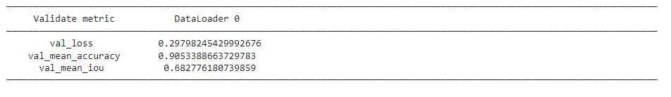
Please note that if we didn't configure the Checkpoint callback the instruction would raise an Exception.
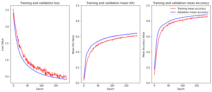
Now if we want to see the plots from our training, we have a csv file saved with our checkpoints that has the history of the training. We can write a function to read it and plot the metrics evolution or we can also use tensorboard.
Since my training stopped many times I couldn't use tensorboard, so I combined all the metrics.csv files and wrote a custom function to plot the loss and the metrics (you can find it in the github repo under utils/utils.py).
If you want to use tensorboard, you can run the two following commands in your notebook
%load_ext tensorboard
%tensorboard --logdir checkpoints/lightning_logs/
Great! our plots look good, we didn't have an overfiting problem : our model is generalizing well in the validation set.
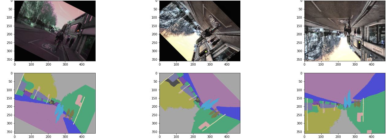
Let's take a look at some predictions. For that we should execute first model.eval() before predicting new images, to stop some layers that behave differently during inference, like BatchNormalization and Dropout. Also use torch.no_grad() to stop gradient computation during inference.
Indeed our predictions are not perfect, but in autonomous vehicules we may tolerate a good enough precision rather than high precision since the goal is to detect the right objects to guide the car.
6.Comparison
While executing this project, I trained three segformer models: (B0, B1 and B2), the results are summarized in the table bellow :
| Model | Mean accuracy | Mean IOU | File size (MB) |
|---|---|---|---|
| SegFormer-B0 | 88% | 64% | 14 |
| SegFormer-B1 | 89% | 67% | 53 |
| SegFormer-B2 | 90% | 68% | 109 |
As shown in the table, although SegFormer-B2 gives the best metrics but it is too big, SegFormer-B1 achieves quiet close results with less parameters, which is why it is the best model in this case.
7. Conclusion
Here are some key take aways from this article:
- Datasets for autonomous driving suffer, usually, from class imbalance
- Deep learning for embedded systems requires a trade off between hardware capabilities, accuracy and model size.
- Data augmentation helps in preventing model overfitting
- Pytorch provides convenient classes to handle data pipeline.
- SegFormer which is based on ViT models, achieves competetive results on semantic segmentation task.
Finally, here are some future ideas to improve the project:
- Try training on different loss (Focal loss for example)
- Try using a different data augmentation scheme
- Try training another ViT model (like MobileVit) and compare it to the results obtained with segformer.
- Try optimizing the training, if possible, by changing the parameters (num_workers, prefetch_factor) of DataLoader class.
References
[1] HOWARD, Andrew G., ZHU, Menglong, CHEN, Bo, et al. Mobilenets: Efficient convolutional neural networks for mobile vision applications. arXiv preprint arXiv:1704.04861, 2017.
[2] XIE, Enze, WANG, Wenhai, YU, Zhiding, et al. SegFormer: Simple and efficient design for semantic segmentation with transformers. Advances in Neural Information Processing Systems, 2021, vol. 34, p. 12077-12090.
[3] MEHTA, Sachin et RASTEGARI, Mohammad. Mobilevit: light-weight, general-purpose, and mobile-friendly vision transformer. arXiv preprint arXiv:2110.02178, 2021.
[4] Julien Fauqueur, Gabriel Brostow, Roberto Cipolla, Assisted Video Object Labeling By Joint Tracking of Regions and Keypoints, IEEE International Conference on Computer Vision (ICCV'2007) Interactive Computer Vision Workshop. Rio de Janeiro, Brazil, October 2007