
Get this book -> Problems on Array: For Interviews and Competitive Programming
In past recent years, the transformer model hit a big success especially in natural language processing applications like language translation and automatic question answering where the model achieved state of the art results. After this success, researches tried to take benefit of this model in many other domains. In 2020 Alexey Dosovitskiy et al [1] used the transformer model to build a new network for image recognition called the vision transformer, that we will try to explain and to implement in this article.
Table of content
- Recalling the transformer model
- The Vision Transformer (ViT) Architecture
- How does it work?
- ViT vs CNNs
- Build and Train ViT using Tensorflow and Keras
- Conclusion
| Point | Vision Transformer |
|---|---|
| What is it? | Transformer model for Image Recognition |
| Formulated in | 2020 |
| Inventor | Alexey Dosovitskiy |
| Main components | Multi-Head Attention, Feed Forward Network |
1. Recalling the transformer model
First let's recall that the transformer model was originally designed for text translation, hence it has an encoder-decoder architecture. Both the encoder and the decoder are composed from a sequencing of layers that are built using two components: multihead-attention and a feed forward network module (ffn) like described in the figure bellow.
Transformer Architecture [2]
These two components play a key role in the success of the transformer model which is why we will explain them in details bellow.
Multi-Head Attention
Before getting to define what a multi-head attention is, let's first understand what do we mean by attention and why we need it.
1. Attention mechanism meaning? There are many different definitions for attention in literature, but in our context it means the ability to dynamically decide on which inputs we want to attend more.
2. Why do we need it? attention was first introduced to improve the encoder decoder architecture for text translation which had a problem of identifying dependencies in long sequences.
3. How is it implemented? The attention mechanism gives a weighted average of sequence elements given as inputs. The weights are computed dynamically using an input query and elements' keys. Ultimately, there are four elements we need to specify:
- Query is a feature vector that describes what would we maybe want to pay attention to.
- Keys is a feature vector that have a key for each input element.
- Values represent the encoded input elements.
- Score Function is the function responsible for computing the weights of inputs using the query and the keys. It can be easily implemented using the dot product like shown in the figure bellow.
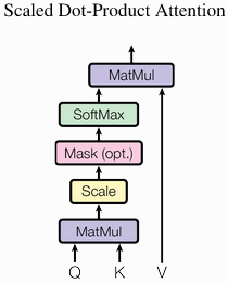
Scaled Dot-Product Attention [2]
The equation used to compute the attention is given by the following equation
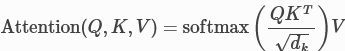
The softmax function is used to compute the weights from the query Q and the keys K .
We divide by √dk (the square root of the keys vector dimensionality) to maintain an appropriate variance of attention values.
V is the values vector.
4. What is multi-head attention?
Multi-head attention uses many triplets of (Q,K,V) instead of only one triplet (Q,K,V). The idea behind it is that one triplet query-key-value gives us the ability to weight elements only in one way in a sequence. However, often one element may have dependencies with more than one element, hence it is useful to have many weights associated with the same element. The architecture of the multi-head attention is shown in the figure bellow.
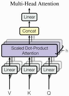
Multi-Head Attention [2]
The following equations describe how multi-head attention is computed
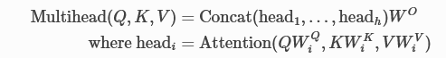
W is a matrix of learnable parameters to weight the different heads.
One crucial characteristic about multi-head attention is that it is permutation-equivariant which means that if the inputs are inverted the result will also be inverted. This characteristic make the attention mechanism and transformer model very powerful because it means that we are looking at the inputs but not their position, which is why the transformer model can be widely applied in other applications.
Feed Forward Network
The feed forward network added after the attention block adds some complexity to the model and allows transformations on each sequence element separately. It can be seen as a post-processing step for the newly computed data by the attention block and also prepares data for the next attention block.
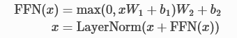
Generally, we use a two layer network with a layer normalization at the end, like shown in the following equations
2. The Vision Transformer (ViT) Architecture
Now that we've seen the crucial components of a transformer, we can move now to understand the vision transformer.
So as we've seen before the transformer was originally proposed to process sets (set of words) because it is permutation-equivariant. But to apply it on sequence data we added a positional encoding for the input features vector and the model learned what to do with it on itself. So why not do the same for images? That is exactly what have been proposed in the paper "An Image is Worth 16x16 Words: Transformers for Image Recognition at Scale". The authors of the paper considered an image as a sequence of patches, and each patch is considered as a word/token and is projected to a feature space. With adding positional encodings and a token for classification on top, we can apply a Transformer as usual to this sequence and start training it for our task. The animation bellow show how this architecture is built.

3. How does it work?
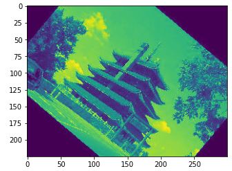
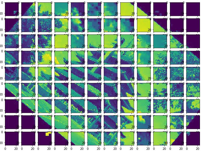
To understand how ViT works, first we should see an image as a sequence of patches. An image of size 225x300X3 for example is divided into patches of 25x25x3 ((225x300)/(25x25) = 108 patches in total).
Once we have the patches (also called tokens), the next step in the classical transformer model is to project them into a certain dimension by adding learnable weights via a Dense layer and then adding positional encoding to learn position dependent information.
A classification token is added to the input sequence. We will use the output feature vector of the classification token for determining the classification prediction.
Then the projected tokens are fed to the Transformer encoder that have the multi-head attention module.
Notice that in this version we are applying the Layer Normalization before the attention mechanism instead of after it. This approach was proposed in 2020 by Ruibin Xiong et al on their paper "On Layer Normalization in the Transformer Architecture" [4]. It turns out that this reorganization supports better gradient flow and removes the necessity of a warm-up stage (start with low learning rate then increase it gradually).
Finally, the transformer encoder outputs feature vector of the CLS token that are fed to an MLP head to map it to a classification prediction. Generally it is implemented with a simple feed forward network or a single linear layer.
4. ViT vs CNNs
Researchers from Google [5] compared the performance of Vit to ResNet on various factors influencing the learning processes of these models. The survey showed the following results:
| ResNet | Vision Transformer | |
|---|---|---|
| Representation structure | Show clear stages in similarity structure. | Has uniform layer similarity structure. |
| Local and Global information | Lower layers of CNNs attend only locally and higher layers attend globally | Vit lower layers have access to both global and local information and higher layers attend only to global information |
| Skip Connections | Skip connections in ResNet are less influential than in ViT | ViT skip connections are highly influential since they enable the clear transition of the class token from lower layers to higher layers |
5. Build and Train ViT using Tensorflow and Keras
In this part of the article at OpenGenus, we will try to implement the vision transformer and apply it on a classification problem.
We will be using the CIFAR100 dataset that is composed of 100 classes. We have about 60000 images of size 32x32.
Note that for simplicity reasons I will not be providing all the code in this section, but I will only provide the essential parts,other details of implementation you can find them in the notebook I will share with you in the end of the article.
Great! let's get started. First we need to implement the function that will extract the patches from a given image. For that we can use the utility function extract_patches provided by Tensorflow.
import numpy as np
import tensorflow as tf
from tensorflow import keras
from tensorflow.keras import layers
import tensorflow_addons as tfa

class Patches(layers.Layer):
    def __init__(self, patch_size):
        super(Patches, self).__init__()
        self.patch_size = patch_size

    def call(self, images):
        batch_size = tf.shape(images)[0]
        patches = tf.image.extract_patches(
            images=images,
            sizes=[1, self.patch_size, self.patch_size, 1],
            strides=[1, self.patch_size, self.patch_size, 1],
            rates=[1, 1, 1, 1],
            padding="VALID",
        )
        patch_dims = patches.shape[-1]
        patches = tf.reshape(patches, [batch_size, -1, patch_dims])
        return patches
Second, the model needs to learn positional information about the image which is why we need to add positional embeddings. For that we need to learn a set of weights to project the patches and then add the positional embeddings.
It is nice to mention that in the original paper an alternative of this method has been used. Instead of using a Dense layer, the authors used a convolutional layer that has a kernel of patch_size then they added the positional embeddings. However, bellow we provide an implementation using the Dense Layer.
class PatchEncoder(layers.Layer):
    def __init__(self, num_patches, projection_dim):
        super(PatchEncoder, self).__init__()
        self.num_patches = num_patches
        self.projection = layers.Dense(units=projection_dim)
        self.position_embedding = layers.Embedding(
            input_dim=num_patches, output_dim=projection_dim
        )

    def call(self, patch):
        positions = tf.range(start=0, limit=self.num_patches, delta=1)
        encoded = self.projection(patch) + self.position_embedding(positions)
        return encoded
Last but not least we can implement the rest of our transformer.
def mlp(x, hidden_units, dropout_rate):
    for units in hidden_units:
        x = layers.Dense(units, activation=tf.nn.gelu)(x)
        x = layers.Dropout(dropout_rate)(x)
    return x

def create_vit_classifier():
    inputs = layers.Input(shape=input_shape)
    # Augment data.
    augmented = data_augmentation(inputs)
    # Create patches.
    patches = Patches(patch_size)(augmented)
    # Encode patches.
    encoded_patches = PatchEncoder(num_patches, projection_dim)(patches)

    # Create multiple layers of the Transformer block.
    for _ in range(transformer_layers):
        # Layer normalization 1.
        x1 = layers.LayerNormalization(epsilon=1e-6)(encoded_patches)
        # Create a multi-head attention layer.
        attention_output = layers.MultiHeadAttention(
            num_heads=num_heads, key_dim=projection_dim, dropout=0.1
        )(x1, x1)
        # Skip connection 1.
        x2 = layers.Add()([attention_output, encoded_patches])
        # Layer normalization 2.
        x3 = layers.LayerNormalization(epsilon=1e-6)(x2)
        # MLP.
        x3 = mlp(x3, hidden_units=transformer_units, dropout_rate=0.1)
        # Skip connection 2.
        encoded_patches = layers.Add()([x3, x2])

    # Create a [batch_size, projection_dim] tensor.
    representation = layers.LayerNormalization(epsilon=1e-6)(encoded_patches)
    representation = layers.Flatten()(representation)
    representation = layers.Dropout(0.5)(representation)
    # Add MLP.
    features = mlp(representation, hidden_units=mlp_head_units, dropout_rate=0.5)
    # Classify outputs.
    logits = layers.Dense(num_classes)(features)
    # Create the Keras model.
    model = keras.Model(inputs=inputs, outputs=logits)
    return model
Finally, we will use Adam with weight decay to optimize our model
def run_experiment(model):
    optimizer = tfa.optimizers.AdamW(
        learning_rate=learning_rate, weight_decay=weight_decay
    )

    model.compile(
        optimizer=optimizer,
        loss=keras.losses.SparseCategoricalCrossentropy(from_logits=True),
        metrics=[
            keras.metrics.SparseCategoricalAccuracy(name="accuracy"),
        ],
    )

    checkpoint_filepath = "/tmp/checkpoint"
    checkpoint_callback = keras.callbacks.ModelCheckpoint(
        checkpoint_filepath,
        monitor="val_accuracy",
        save_best_only=True,
        save_weights_only=True,
    )

    history = model.fit(
        x=x_train,
        y=y_train,
        batch_size=batch_size,
        epochs=num_epochs,
        validation_split=0.1,
        callbacks=[checkpoint_callback],
    )

    model.load_weights(checkpoint_filepath)
    _, accuracy = model.evaluate(x_test, y_test)
    print(f"Test accuracy: {round(accuracy * 100, 2)}%")

    return history


vit_classifier = create_vit_classifier()
history = run_experiment(vit_classifier)
Outputs:
Test accuracy: 54.65%
Notice that this isn't the best result for classifying CIFAR100, but that's a totally fine result because the authors of ViT mentioned that their model outperforms CNNs when it is trained on large datasets. The results that the authors got on their paper were achieved after training ViT on JFT-300M dataset, then fine-tuning it on the target dataset.
To get access to the full code used in this article you can click here.
6. Conclusion
To wrap up what have been covered in this article, here are some key points to keep in mind about the vision transformer:
- The vision transformer sees images as a sequence of patches.
- ViT learns from scratch the positional dependency between the patches
- ViT uses multi-head attention modules that enables the lower layers to attend to both global and local informations.
- ViT has a higher precision rate on a large dataset with reduced training time.
References
[1] DOSOVITSKIY, Alexey, BEYER, Lucas, KOLESNIKOV, Alexander, et al. An image is worth 16x16 words: Transformers for image recognition at scale. arXiv preprint arXiv:2010.11929, 2020.
[2] VASWANI, Ashish, SHAZEER, Noam, PARMAR, Niki, et al. Attention is all you need. Advances in neural information processing systems, 2017, vol. 30.
[3] WANG, Phil. Lucidrains/VIT-pytorch: Implementation of vision transformer, a simple way to achieve SOTA in vision classification with only a single transformer encoder, in Pytorch. GitHub [online]. 28 March 2021. Available from: https://github.com/lucidrains/vit-pytorch
[4] XIONG, Ruibin, YANG, Yunchang, HE, Di, et al. On layer normalization in the transformer architecture. In : International Conference on Machine Learning. PMLR, 2020. p. 10524-10533.
[5] RAGHU, Maithra, UNTERTHINER, Thomas, KORNBLITH, Simon, et al. Do vision transformers see like convolutional neural networks?. Advances in Neural Information Processing Systems, 2021, vol. 34, p. 12116-12128.