
Convex optimization can be used to formulate many of the latest issues in statistics and machine learning. It is becoming more crucial to be able to tackle issues with a very large number of features, training samples, or both as a result of the increase in size and complexity of modern datasets. Therefore, it is either essential or at the very least extremely desired that these datasets be collected or stored decentralizedly, along with the associated distributed solution techniques. Distributed convex optimization, and in particular, large-scale issues occurring in statistics, machine learning, and related fields, are particularly suited to the Alternating Direction Method of Multipliers (ADMM).
Table of contents
- Introduction
- Dual Ascent
- Dual Decomposition
- Augmented Lagrangians and Method of Multipliers
- Alternating Direction Method of Multipliers
- Form 1
- Form 2
Introduction
The technique was created in the 1970s, though its origins date back to the 1950s. It is similar to or interchangeable with many other algorithms, including dual decomposition, the multiplier method, Douglas-Rachford splitting, Spingarn's partial inverses method, Dykstra's alternating projections, Bregman iterative algorithms for problems, proximal methods, and others. We explore applications to a wide range of statistical and machine learning issues of current interest, including the lasso, sparse logistic regression, basis pursuit, covariance selection, support vector machines, and many more, after briefly reviewing the theory and history of the approach.
A straightforward and effective iterative approach for convex optimization issues is ADMM. In comparison to traditional approaches, it solves multivariable problems over 80 times quicker. In a single framework, ADMM takes the place of linear and quadratic programming.
- The L0 norm is the number of non-zero elements in a vector.
The L0 norm is popular in compressive sensing which tries
to find the sparsest solution to an under-determined set of equations.
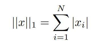
- The L1 norm that is calculated as the sum of the absolute values of the vector is mathematically represented as,
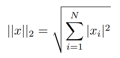
- The L2 norm is calculated as the square root of the sum of the squared vector values. The max norm that is calculated
as the maximum vector values.
With these basic terms reviewed, we can advance to understand step by step process of how ADMM was arrived at.
Dual Ascent
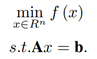
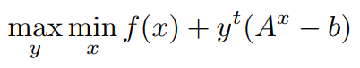
Let us consider the following Convex constrained optimization problem:
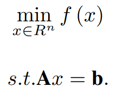
Here, A ∈ R^m×n, b ∈ R^m, and f: R^n → R is a convex function. y is a Lagrange multiplier Lagrange
we can dual function for the above optimization problem as,
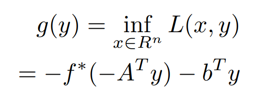
Here f∗ is a convex conjugate of f. Now, we have to optimize the dual function.
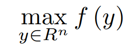
Considering that strong duality holds for the above. The primal and dual solutions are the same. with this primal solution, x∗ can be recovered from dual optimal solution y∗
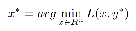
Now, Coming to the Dual Ascent Method, we use the gradient ascent method to find out the residual for the equality constraint Updating of Variables can be done in the following way,
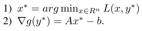
Now the Iterative updates are,
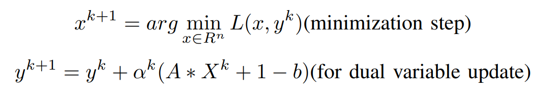
where α^k is the step size. Finally, this algorithm is called ‘dual ascent’ since the dual function increases in each step (g(y^k+1) > g(y^k)) with an appropriate choice of α^k
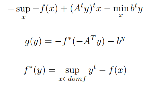
Deriving the Dual Function
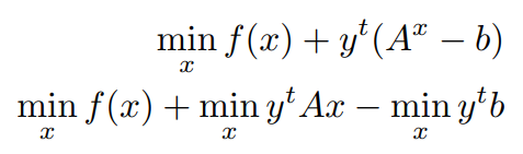
Now let us Understand How we got the dual,
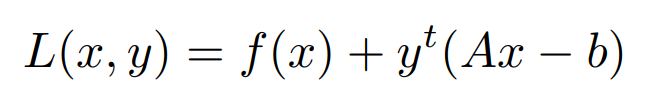
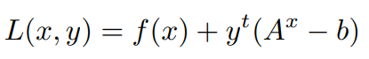
Formulating the Lagrangian for the Above Equation,
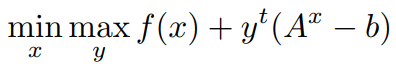
From the Above Equation, we can understand that we have maximized the Lagrangian Multiplier y and minimize the objective function,
by Strong Duality,
Now let us Expand the inner min of the above Function,
using,
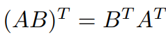
we get,
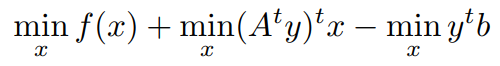
Now we have to convert the min formulation to supremum Formulation,
From Dual Ascent we want to consider the movement of assumed solution x towards optimal solution x* iteratively for a given optimization problem.
Dual Decomposition
The major benefit of the dual ascent method is that it can lead to a decentralized algorithm. Suppose objective f is separable, let’s breakdown the objective function f(x) as,
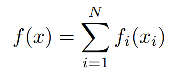
where x = [x1, x2, · · · , xN ] and each xi ∈ R^ni
is a sub-vector of x. Similarly, partitioning A = [A1, A2, · · · , AN ], we get
Clearly, the x-minimization step in the Dual Ascent Method has now been split into N separate problems that can be solved parallelly. Hence, the update steps are,

The minimization step obtained is solved in parallel for each i = 1, 2, · · ·, N. Consequently, this decomposition in the dual ascent method is referred to as the dual decomposition.
From Dual Decomposition we want to consider the minimization step to be separable from the rest of the general equation which allows parallelization, which results in faster convergence.
Augmented Lagrangians and Method of Multipliers
The convergence of the dual ascent algorithm is based on assumptions such as strict convexity or finiteness of f. To avoid such assumptions and ensure the robustness of the dual ascent algorithm, Augmented Lagrangian methods were developed.
Purpose of addition of Augmented term
The Augmented Lagrangian terms represent a Smooth function. When a smooth function is added to a non-smooth function the resulting function is smooth. In the case of the lagrangian fucntion, it allows for the application of ADMM. Hence, the Addition of Augmented Lagrangian is justified.
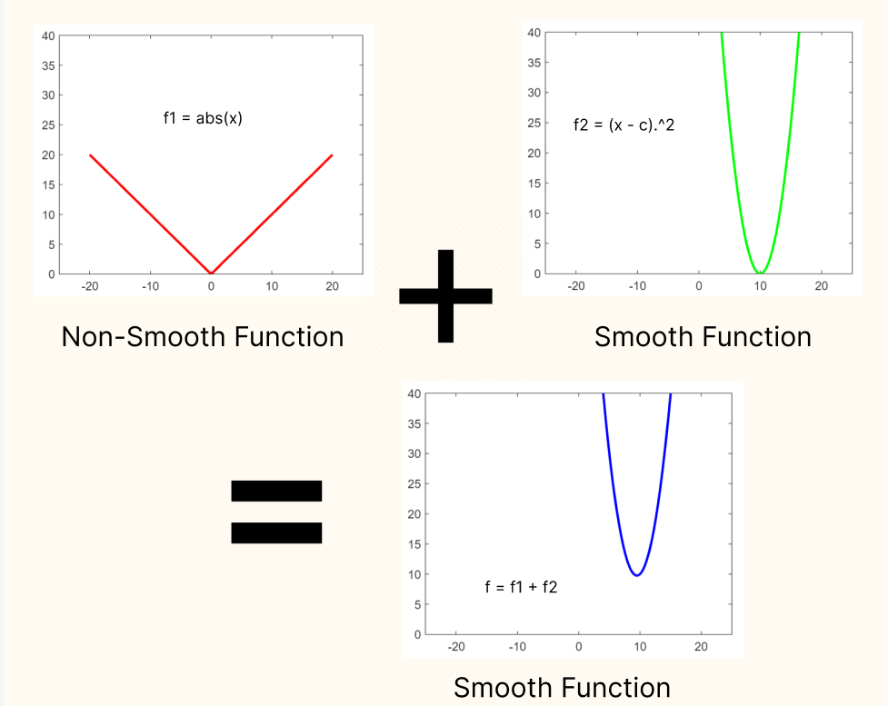
the code for this plot is as simple as,
x = linspace(-20,20,400)
c = 10

f1 = abs(x)

f2 = (x - c).^2

f = f1 + f2;
hold off
a = plot(x, f1)
a.LineWidth = 2
a.Color = "Red"
xlim([-25,25])
ylim([0, 40])

b = plot(x, f2)
b.LineWidth = 2
b.Color = "Green"
xlim([-25,25])
ylim([0, 40])

c = plot(x, f)
c.LineWidth = 2
c.Color = "blue"
xlim([-25,25])
ylim([0, 40])
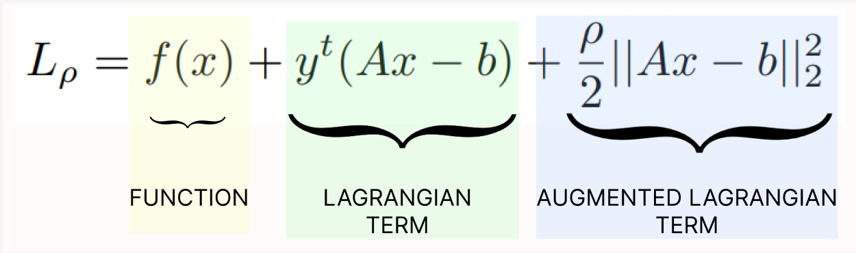
Here ρ > 0 is called the penalty parameter. This augmented Lagrangian can be viewed as the unaugmented Lagrangian of the problem,
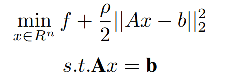
Here above and original problems are similar because for any feasible x, the term (ρ/2)||Ax − b||2^2 becomes zero. The associated dual to the above representation is,
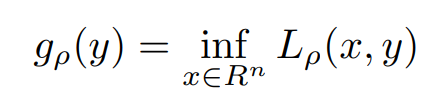
Adding (ρ/2)||Ax − b||2^2 to f(x) makes gρ differentiable under milder conditions than on the original problem.
Next, the gradient of the augmented dual function is found similarly as above. Applying the dual ascent algorithm to the modified problem above gives
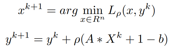
The Above equations are called Method of Multipliers: This method is the same as the standard dual ascent, with the penalty parameter ρ used in place of step size α^k. The advantage of the method of multipliers is that it converges under far more general conditions than the dual ascent.
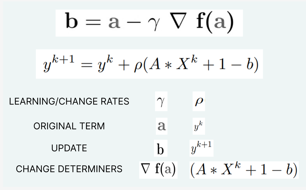
This is blatantly similar to the Gradient Descent equation,
Alternating Direction Method of Multipliers
Alternating Direction Method of Multipliers or ADMM is an algorithm which tries to solve the problem faced using the Method of
Multipliers by combining the decomposability of dual ascent with the Greater convergence properties of the Method of multipliers.
ADMM is a simple and powerful iterative algorithm for convex optimization problems. It is almost 80 times faster for
multivariable problems than conventional methods. ADMM replaces linear and quadratic programming in a single framework.
ADMM solves the problems in particular form and adheres to two forms
Form 1
Consider the unconstrained problem,
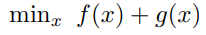
Where, f: R^n → R, g: R^n → R are convex functions.
Now the alternating direction method of multipliers (ADMM) is defined as,
where k is the iteration counter
Derivation For Form I
Here we are changing the problem by introducing a new variable z and also importing a constraint. The variable has been
split into two variables x and z. Therefore the number of variables has been doubled but the optimization problem remains
the same. Basically converting an unconstrained problem into a constrained one and trying to solve that by using the augmented
Lagrangian
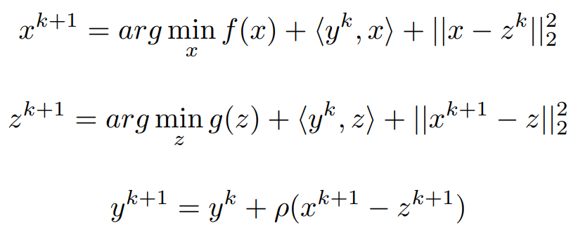
Now our Optimization Problem changed to,
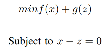
And this is Equivalent to minimizing f(x) + g(x)
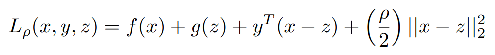
Now let's Write Lagrangian For Above Equation

Where ρ >0 is a parameter and y ∈ Rn is the Lagrangian dual variable
another term (ρ/2) ||Ax − b||2^2
called augmented Lagrangian is also added. This will be a highly convex function and so
the addition of this extra term increases the convexity of our original problem and it will converge quickly to the solution. So now there are three variables x,y, and z
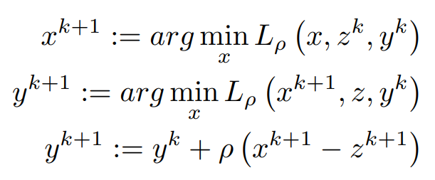
In each iteration, x and Z are using Previous values from Primal Solution and Y is accelerating the term
Now we are trying to convert Lagrangian into proximal Form
For x and z values are Randomly chosen and trying to minimize the Lagrangian,
Arranging all the linear terms into Quadratic form,
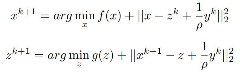
Now Let us make some assumptions that we will use those make it to proximal Form.
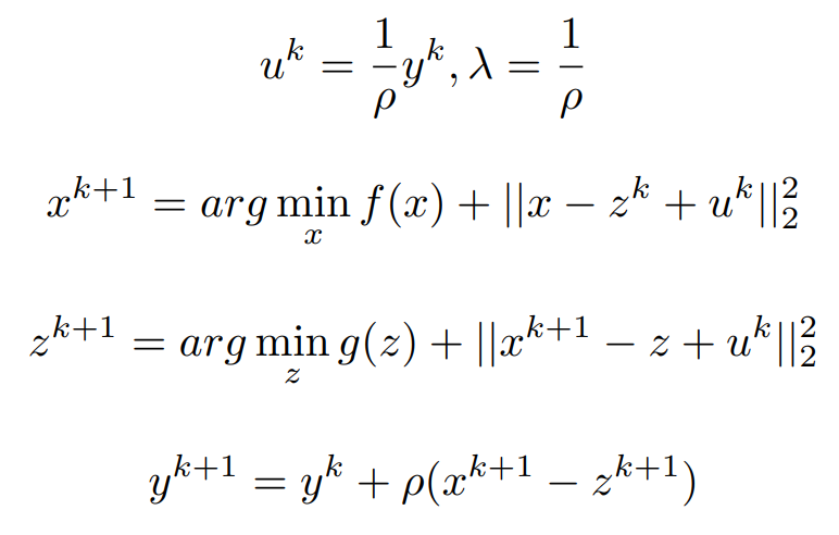
The Proximal form is given by,
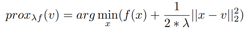
Now Let us Write Everything into proximal Form,
Our New Equation is below,
equivalently,
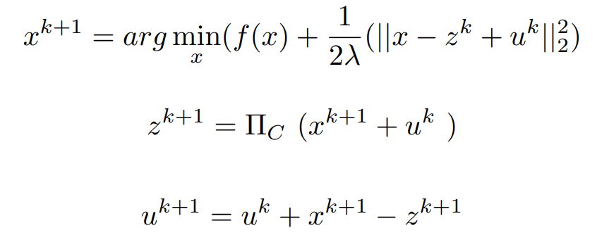
Form 2
Consider the constrained optimization problem,
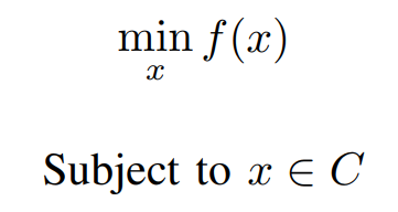
where f and C are Convex
The Problem is Now written in the format of ADMM,
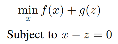
Where g(.) is an indicator function of and is defined as,
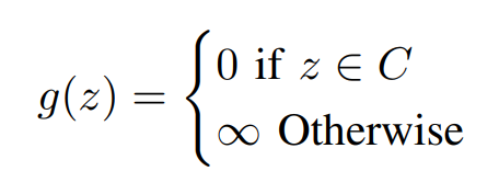
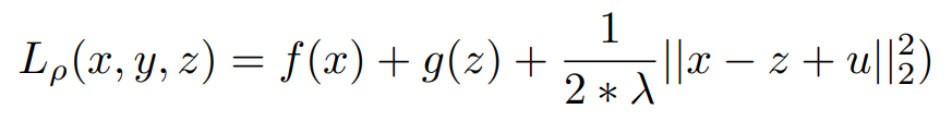
In the Above Equation, all our constraints are represented in an indicator function G(z) in a different variable and the variables are made equal by introducing a new constraint. Now Lets us Consider the augmented Lagrangian function,
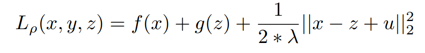
According to the definition of the indicator function, if g(z) = 0 means we are actually minimizing the original function. So when the algorithm proceeds at any stage we are forced to choose a z, which is an element of C. If it is not, then, Z = ∞ and further optimization is not possible. For Minimizing the x we know the Solution of z^k and y^k.
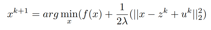
Now ,We Have to be Care-full for Updating the Value of Z .Because if Z = x + u ,means 1/2λ(||x − z^k + uk||22) = 0, but g(z) = ∞. Here going for the concept of projection. In order to choose z which minimizes the Lagrangian the concept of
projection is used.
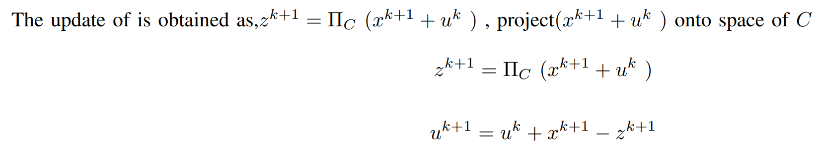
If x − z = 0 then u^k+1 = u^k
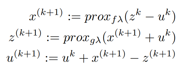
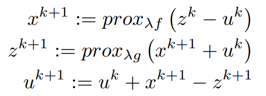
Finally, the Iterative Steps are :
After carefully comprehending the ADMM fundamentals, we may use ADMM to tackle L1 Optimization issues. This enables us to demonstrate the Solutions' practical usefulness.
References
A substantial portion of the ADMM derivation is derived from L1-Norm problems solved using ADMM