
Open-Source Internship opportunity by OpenGenus for programmers. Apply now.
Reading time: 30 minutes | Coding time: 20 minutes
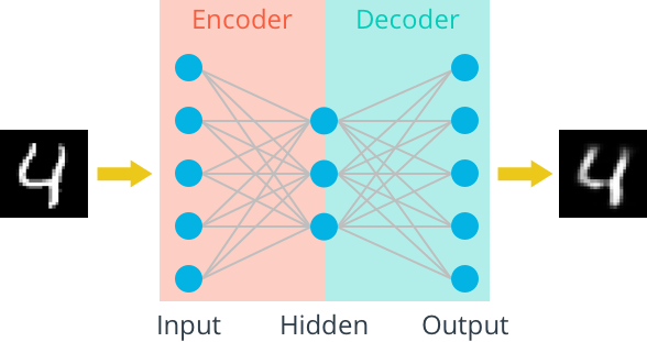
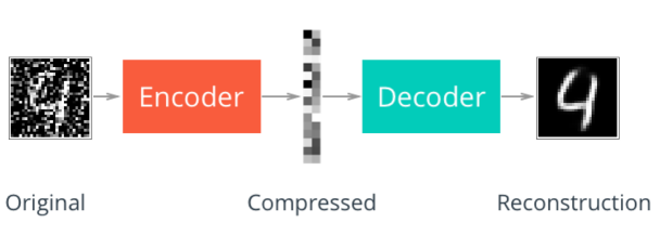
An autoencoder is a neural network that learns data representations in an unsupervised manner. Its structure consists of Encoder, which learn the compact representation of input data, and Decoder, which decompresses it to reconstruct the input data.
For example, in case of MNIST dataset,

Linear autoencoder
The Linear autoencoder consists of only linear layers. Let's build a simple autoencoder for MNIST in PyTorch where both encoder and decoder are made of one linear layer. First, the data is passed through an encoder that makes a compressed representation of the input. Then, this representation is passed through a decoder to reconstruct the input data.
import torch.nn as nn
import torch.nn.functional as F

class Autoencoder(nn.Module):
    def __init__(self, encoding_dim):
        super(Autoencoder, self).__init__()
        ## Encoder ##
        # linear layer (784 -> encoding_dim)
        self.fc1 = nn.Linear(28 * 28, encoding_dim)

        ## Decoder ##
        # linear layer (encoding_dim -> input size)
        self.fc2 = nn.Linear(encoding_dim, 28*28)

    def forward(self, x):
        x = F.relu(self.fc1(x))
        # output layer (sigmoid for scaling from 0 to 1)
        x = F.sigmoid(self.fc2(x))
        return x

encoding_dim = 32
model = Autoencoder(encoding_dim)
Let's load the datasets and train the model.
import torch
import numpy as np
from torchvision import datasets
import torchvision.transforms as transforms

# load the training and test datasets
train_data = datasets.MNIST(root='data', train=True, download=True, transform=transforms.ToTensor())
test_data = datasets.MNIST(root='data', train=False, download=True, transform=transforms.ToTensor())
batch_size = 20
train_loader = torch.utils.data.DataLoader(train_data, batch_size=batch_size)
test_loader = torch.utils.data.DataLoader(test_data, batch_size=batch_size)

# loss function
criterion = nn.MSELoss()
optimizer = torch.optim.Adam(model.parameters(), lr=0.001)
n_epochs = 20

for epoch in range(1, n_epochs+1):
    train_loss = 0.0

    for data in train_loader:
        images, labels = data
        # flatten images
        images = images.view(images.size(0), -1)
        optimizer.zero_grad()
        # forward pass
        outputs = model(images)
        # calculate the loss
        loss = criterion(outputs, images)
        # backward pass + optimization
        loss.backward()
        optimizer.step()
        # update running training loss
        train_loss += loss.item()*images.size(0)

    # print avg training statistics
    train_loss = train_loss/len(train_loader)
    print('Epoch: {} \tTraining Loss: {:.6f}'.format( epoch, train_loss))
Now, let's see the output images.
dataiter = iter(test_loader)
images, labels = dataiter.next()

images_flatten = images.view(images.size(0), -1)
# get sample outputs
output = model(images_flatten)
images = images.numpy()
output = output.view(batch_size, 1, 28, 28)
output = output.detach().numpy()

# plot the first ten input images and then reconstructed images
fig, axes = plt.subplots(nrows=2, ncols=10, sharex=True, sharey=True, figsize=(25,4))
for images, row in zip([images, output], axes):
    for img, ax in zip(images, row):
        ax.imshow(np.squeeze(img), cmap='gray')
        ax.get_xaxis().set_visible(False)
        ax.get_yaxis().set_visible(False)
Input images
Reconstructed images

Convolutional autoencoder
In Convolutional autoencoder, the Encoder consists of convolutional layers and pooling layers, which downsamples the input image. The Decoder upsamples the image. The structure of convolutional autoencoder looks like this:
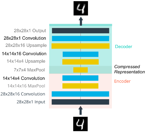
Let's review some important operations.
Downsampling
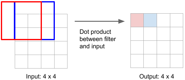
The normal convolutional operation (without stride) gives the same-size output image as input image e.g. 3x3 kernel (filter) convolution on 4x4 input image with stride 1 and padding 1 gives the same-size output.
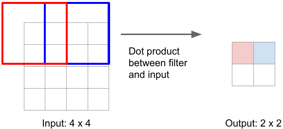
But strided convolution results in downsampling i.e. reduction in size of input image e.g. 3x3 convolution with stride 2 and padding 1 convert image of size 4x4 to 2x2.
Upsampling
One of the ways to upsample the compressed image is by Unpooling (the reverse of pooling) using Nearest Neighbor or by max unpooling.
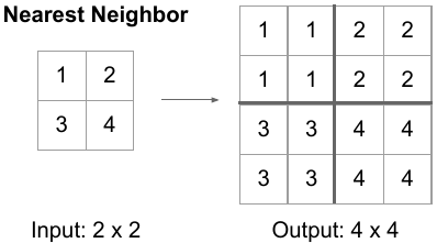
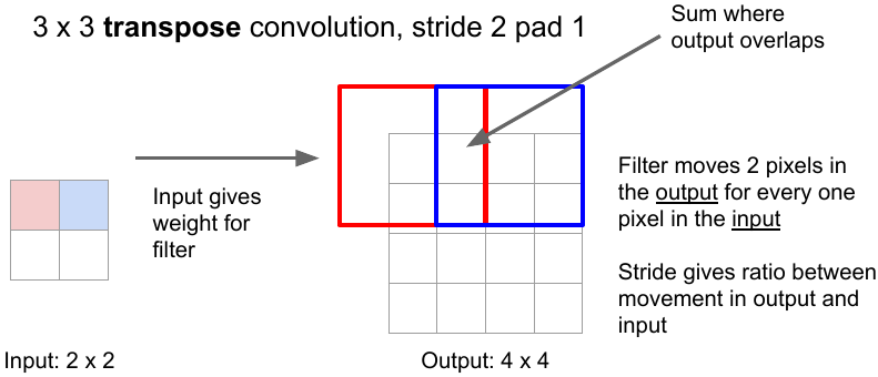
Another way is to use transpose convolution. The convolution operation with strides results in downsampling. The transpose convolution is reverse of the the convolution operation. Here, the kernel is placed over the input image pixels. The pixel values are multiplied successively by the kernel weights to produce the upsampled image. In case of overlapping, the values are summed. The kernel weights in upsampling are learned the same way as in convolutional operation that’s why it’s also called learnable upsampling.
One other way is to use nearest-neighbor upsampling and convolutional layers in Decoder instead of transpose convolutional layers. This method prevents checkerboard artifacts in the images, caused by transpose convolution.
Denoising autoencoders
The denoising autoencoder recovers de-noised images from the noised input images. It utilizes the fact that the higher-level feature representations of image are relatively stable and robust to the corruption of the input. During training, the goal is to reduce the regression loss between pixels of original un-noised images and that of de-noised images produced by the autoencoder.
There are many other types of autoencoders such as:
- Variational autoencoder (VAE)
- Denoising autoencoder
- Sparse autoencoder
- Contractive autoencoder (CAE)
