Back-propagation is the most widely used algorithm to train feed forward neural networks. The generalization of this algorithm to recurrent neural networks is called Back-propagation Through Time (BPTT). Although BPTT can also be applied in other models like fuzzy structure models or fluid dynamics models [1], in this article the explanations are based on the application of BPTT on recurrent neural network to make understanding it more easier.

Table of content

1. The math behind BPTT
2. Variations of BPTT
3. Conclusion

1. The math behind BPTT

Before we start diving into the calculations, we will start by defining a simple recurrent neural network and unfolding it to explain what happens in each time step t during the execution of back-propagation.

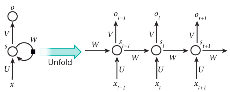
As you may have noticed in the figure, we have three weight matrices involved in the calculation of each output o at time step t :
U are the weights associated with the inputs x_t.
W are the weights associated with the hidden state of the RNN.
V are the weights associated with the outputs of the RNN.

Training a neural network requires the execution of the forward and back-propagation pass.
The forward pass involves applying the activation functions on the inputs and returning the predictions at the end , while the back-propagation pass involves the calculation of the objective function gradients' with respect to the weights of the network to finally update those weights.

So how many gradient equations do we need to compute in our simple RNN?
We have three weight matrices (U, W and V), so we need to compute the derivative of the objective function with respect to three weights.

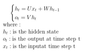
Before we start computing the derivatives, let's start by recalling the equations for the forward pass.
Note:
For simplicity reasons, we assume that the network doesn't use bias and that the activation function is the identity function (f(x)=x).

We will consider the objective function L the loss l over time steps from the beginning of the sequence. It is defined by the following equation

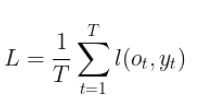
Now that the objective function has been defined, we can start explaining the computations made in the BPTT algorithm.
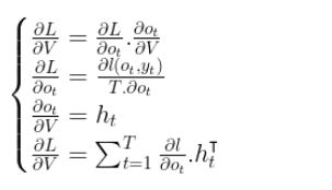
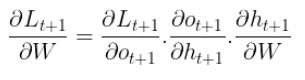
Looking to the top of our RNN architecture, the first derivative that we need to compute is the derivative with respect to the weights V that are associated with the outputs o_t. For that we will be using the chain rule.

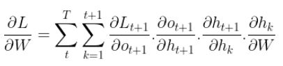
Looking again to the architecture of the network, the next gradient we should compute is the one with respect to W (the weights of the hidden state).
For that let's first consider the gradient of L at time step t+1 with respect to the weights W, using the chain rule we get

From the equations of the forward pass, we know that the hidden state at time step t+1 is dependent on the hidden state at time step t, with that in mind the above equation become

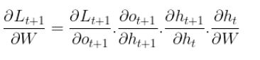
However, here the things become tricky because also the hidden state at time step t is dependent on all the past hidden states, so we need their gradients with respect to W and for that we will be using the chain rule for multi-variable function.

Reminder:
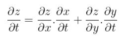
The multi-variable chain rule is defined as follow:
Let z = f(x,y) where x and y themselves depend on one or more variables.
The multi-variable chain rule allow us to differentiate z with respect to any of the variable that are involved.

Let x and y be differentiable at t and suppose that z = f(x,y) is differentiable at the point (x(t),y(t)). Then z = f(x(t),y(t)) is differentiable at t and :

So the equation computed before becomes :

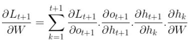
Great! now it becomes easy for us to compute the gradient of the objective function L with respect to W for the whole time steps

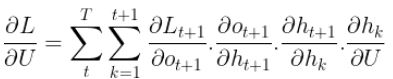
Finally, we need to compute the gradients with respect to the weights U that are associated with the inputs.
Since U appears also in the equation of the hidden state just like W, using the same pattern to compute the gradients with respect to W, we get the gradients with respect to U as follow :

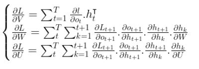
Awesome! we are now done with the computations, here are the three gradient equations we computed :

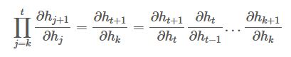
One final thought is: have you noticed that the gradient of the hidden state at time step t+1 with respect to the hidden state at time step k is in itself a chain rule?! If so can you elaborate the two last gradients we computed?
Using the chain rule we have :

In the next section we will see how computing this equation in practice may be problematic.

2. Variations of BPTT

There are 3 Variations of BPTT:

• Full BPTT
• Truncated Time steps (TBPTT)
• Anticipated Reweighted Truncated Backpropagation (ARTBP)

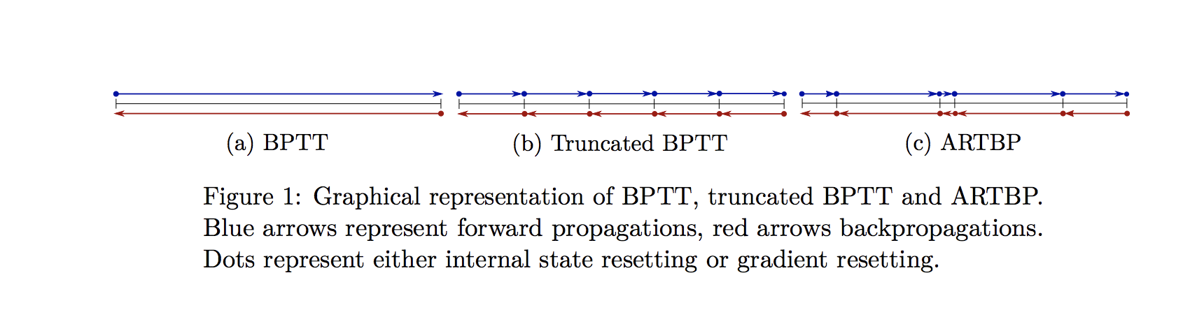
Full BPTT

The above explained method is the full version of back-propagation through time, and actually this version is never used in practical cases because it involves many computations and the equation we gave at the end of the previous paragraph makes the computations very slow and the gradients may either vanish or explode, but why? when the gradients are smaller than 1 the given multiplication makes the results even smaller causing the gradients to vanish, on the other hand when the gradients are big the given multiplications cause the gradients to explode. Knowing that any change in the initialization may lead to one of these two situations, training the RNN then becomes very problematic.

To reduce the computations caused by Full BPTT, researchers suggested to truncate the sums to a certain time step, this method is explained in the two upcoming paragraphs and for the problem of vanishing/and exploding gradients it is suggested to clip the gradients.

Truncated Time steps

The idea is to stop computing the sum of gradients after time step τ, this leads to an approximation of the true gradients and gives quite good results in practice. This version of BPTT is called Truncated Backpropagation Through Time (referred as TBPTT) [2]. As a consequence to this method, the model starts focusing on short term influence rather than long-term ones and with that the model becomes biased. To solve this problem, the researchers suggested to use subsequences with variable length instead of using fixed length subsequences. This method is explained in the following paragraph.

Randomized Truncations

The idea is to use a random variable to generate variable truncation
lengths together with carefully chosen compensation factors in the back-propagation equation. This method is called Anticipated Reweighted Truncated Backpropagation (ARTBP) [3], it keeps the advantages of TBPTT while reducing the bias of the model.

BPTT	TBPTT	ARTBP
Saves all the inputs and activation outputs during the forward pass for use in gradient computations It is computationally expensive and memory intensive, particularly in character language models. The gradient values at time t’ used in every time step t if t < t’.	The input is treated as a fixed length subsequences In gradient computation, the computed gradient values are dropped at the end of every subsequence in back-prop. Introduces bias to the model.	Uses variable length subsequences with weighted factors in backpropagation equation to reduce bias. Although in theory, ARTBP looks better than TBPTT, in practice this method doesn't seem to generate much better results than TBPTT.

3. Conclusion

To wrap up what have been covered in this article, here are some of the key takeaways:

• Backpropagation through time is an algorithm used to train sequential models especially RNNs.
• Truncating time steps are needed in practice to cut off the computation and the excess use of memory.
• For efficient computation, intermediate values are cached during backpropagation through time.
• High power matrices may lead to vanishing or exploding eigenvalues which in turn cause vanishing or exploding gradients.

References

[1] WERBOS, Paul J. Backpropagation through time: what it does and how to do it. Proceedings of the IEEE, 1990, vol. 78, no 10, p. 1550-1560.
[2] JAEGER, Herbert. Tutorial on training recurrent neural networks, covering BPPT, RTRL, EKF and the" echo state network" approach. 2002.
[3] TALLEC, Corentin et OLLIVIER, Yann. Unbiasing truncated backpropagation through time. arXiv preprint arXiv:1705.08209, 2017.