In this article, we will be walking through the concept behind Bellman's Optimality equation, and how it is used in the case of Reinforcement Learning.

$$V\left(s\right){=}_a^{\max }\left(R(s,a)\right)+\gamma V(s\text{'}))-->$$ Bellman's equation for deterministic environment

Bellman’s optimality equation:

$$V^{*}(s)={\displaystyle \sum _a\pi (a|s)}.{\displaystyle \sum _{s\text{'}}P(s\text{'}|a)\left[E(r|s,as\text{'})+\gamma V^{*}(s\text{'})\right]}$$

Bellman’s equation is one amongst other very important equations in reinforcement learning.
As we already know, reinforcement learning RL is a reward algorithm that tries to enable an intelligent agent to take some actions in an environment, in other to get the best rewards possible – it seeks to maximize our long-term rewards.

The bellman’s equation seeks to estimate whether actions taken was able to really return the maximum rewards as expected, in other words, it tries to hint us the kind of rewards we could expect if we take certain best actions now based on our present state, and if we continue with such actions in the future steps.

For the deterministic environment, bellman’s equation can be viewed thus:

• The max_a function tries to choose actions that will get the maximum rewards.
• The discount rate γ,is basically a hyper-parameter which helps in adjusting and suiting our decisions process, it shows how valuable the rewards will be for the long-term or for the short-term; hence it guides the agent on whether to focus on long or short-term rewards.
• The rest part of the quation centers on calculating the rewards.

The bellman’s equation is a recursive type - calls itself during execution of the commands; that is, it repeats actions so many times before giving out the desired output.

Summary for the deterministic equation:
A Step is taking, resulting to an action, the action leads to a new state, new state gives a new reward and an episode ends….at this point, we backtrack – we apply the discount factor γ , then we utilize the max_a function to choose actions that gave us the maximum rewards, then we calculate the rewards using the R(s,a) function ”

Important terminologies used herein:
Policy π = this tells the agent what best action to taking in a given state or situation.

Value function:

$$V^{\pi }(s)=E(G_t|s_t=s)$$ – this seeks to estimate how suitable is it for an agent to be in a particular state, and how appropriate the action of an agent best suits a given state or situation. From here, we can see that the way an agent tends to act, in directly influenced by the policy it is following, consequently, the value function is defined with respect to the policies. **Discounted return**: This is intended to take rewards that comes first in the short term, and not having to wait for cumulative future reward to be returned. It concerns itself with returns that falls within the discount rate γ– values from 0 – 1. It helps to converge our returned rewards within a chosen range of the discount rate/factor. let's review the relationships on how the returns at successive time steps are related to each other: $$\begin{array}{l}{G}_t=R_{t+1}+\gamma R_{t+2}+{\gamma }^2{R}_{t+3}+{\gamma }^3{R}_{t+4}\mathrm{......}\\ G_t=R_{t+1}+\gamma (R_{t+2}+\gamma R_{t+3}+{\gamma }^2{R}_{t+3}\mathrm{.....})\\ G_t=R_{t+1}+\gamma G_{t+1}\end{array}$$

Hence , we can see that -

$$G_t=R_{t+1}+{\gamma }^2{R}_{t+2}+{\gamma }^3{R}_{t+3}\mathrm{.......}+{\gamma }^T{R}_T={\displaystyle \sum _{k=0}^{\infty }{\gamma }^k}{R}_{t+k}={\displaystyle \sum _{\Delta t=0}^{\infty }{e}^{-\Delta t/\pi }}{R}_{t+\Delta t}$$

Let’s now look into how to derive the Bellman’s Optimality Equation:

Proof of Bellman’s Equation

$$V^{\pi }(s)=E(G_t|s_t=s)$$

; where E is the expectation, Rt = the return in time state, s t = the state in time,

$$\pi =Policy-->(a-->s)$$

G t = return of reward =

$$G_t=R_{t+1}+\gamma R_{t+2}+{\gamma }^2{R}_{t+3}+{\gamma }^3{R}_{t+4}\mathrm{......}$$

and

$$\gamma =discount\_rate:0\le \gamma \ge 1$$

Now considering Gt,

$$\begin{array}{l}{G}_t=R_{t+1}+\gamma (R_{t+2}+\gamma R_{t+3}+{\gamma }^2{R}_{t+3}\mathrm{.....})\\ G_t=R_{t+1}+\gamma G_{t+1}\end{array}$$

Hence,

$$V^{\pi }(s)=E[R_{t+1}+\gamma (G_{t+1})|s_t=s]$$ meaning – the expectation of the returns, given the time state St = state S

Illustrative Diagram

$$$$
(s)−−−>(s')

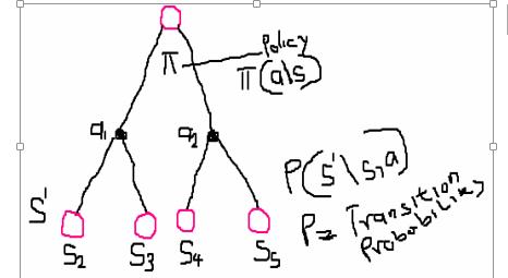
Note: a\s = action, given the very state.
What happens here is this:
The agent starts at a state s, follows a policy π, takes an action a, and goes into a new state s'.
The probability of the agent taken an action using a policy =

$$\pi (a|s),$$

The probability of taken the next action in the new state

$$S\text{'}=P(s\text{'}|s,a)$$

Where P is a transitional probability – and it is environment dynamic.

Likewise, the probability of moving from S to S5 taken action a2:

$$P{s}_5{a}_2=\pi (a_2|s).P(s_5|s,a_2)$$

furthermore, the probability of moving from S to any of the action S' is:

$${\rm P}={\displaystyle \sum _{a\epsilon A}\pi (a|s)}.{\displaystyle \sum _{s\text{'}\epsilon S}P(s\text{'}|s,a_2)}$$

Our value function is :

$$V^{\pi }(s)={\rm P}.E[R_{t+1}+\gamma G_{t+1}|s_{t+1}=s\text{'}]$$

Now substituting for P into the value function;

$$V^{\pi }(s)={\displaystyle \sum _a\pi (a|s)}.{\displaystyle \sum _{s\text{'}}P(s\text{'}|a)}.E[R_{t+1}+\gamma G_{t+1}|s_{t+1}=s\text{'}]$$

Now considering the expectation and taking E inside the equation, we get

$$=E(r|s,as\text{'})+\gamma E[G_{t+1}|s_{t+1}=s\text{'}]$$

Going further, we know that –

$$\begin{array}{l}{V}^{\pi }(s)=E[G_{t+1}|s_{t+1}=s\text{'}]\\ \therefore E(r|s,as\text{'})+\gamma E[G_{t+1}|s_{t+1}=s\text{'}]=E(r|s,as\text{'})+\gamma V^{\pi }(s)\end{array}$$

Consequently, Bellman’s equation for policy π, can then be written as:

$$V^{\pi }(s)={\displaystyle \sum _a\pi (a|s)}.{\displaystyle \sum _{s\text{'}}P(s\text{'}|a)}.E[(r\backslash s,as\text{'})+\gamma V^{\pi }(s)]$$

Furthermore, we know that:

$$\begin{array}{l}\pi =highest\_reward-->Optimal\_Policy\\ V^{*}(s){=}_{\pi }^{\max }{V}^{\pi }(s)-->Optimal-value\_function\end{array}$$

Finally, this leads to Bellman’s optimal equation -

$$V^{*}(s)={\displaystyle \sum _a\pi (a|s)}.{\displaystyle \sum _{s\text{'}}P(s\text{'}|a)}.\left\{E(r|s,as\text{'})+\gamma V^{*}(s\text{'})\right\}$$

We could also look at this from the Q – function perspective –

$$Q^{*}(s,a)=OptimalQ\_function$$ $$\begin{array}{l}But\\ V^{*}(s)={\displaystyle \sum _a\pi (a|s)}.Q^{*}(s,a)\end{array}$$

Therefore, Bellman’s Equation using Q-function –

$$Q^{*}(s,a)={\displaystyle \sum _{s\text{'}}P(s\text{'}|a)}.\left\{E(r|s,as\text{'})+\gamma {\displaystyle \sum _a\pi (a|s\text{'})}.Q^{*}(s\text{'},a)\right\}$$

From the insight rendered thus far, there is no doubt you have gotten an idea behind the Bellman's Optimality equation, and how it is used in the case of Reinforcement Learning. Thank you for enjoying this article at OpenGenus.