
In Natural Language Processing (NLP), Document Similarity Calculation is a crucial task that involves checking how similar two or more documents are. This article shall focus on its use cases, the concept behind different techniques of document similarity, and their implementations in Python.
Use Cases of Document Similarity

-
Search Engines- Document Similarity is used by search engines to return documents that are related to the user's search query. When a user inputs a search query, for example, the search engine compares it to the items in its index and returns the documents that are most similar to the query.
-
Plagiarism Detection- Document Similarity is used by plagiarism detection algorithms to identify instances of plagiarism in documents. When a document is submitted to a plagiarism detection system, it is compared to the set of existing documents in order to find any similarities. The system classifies the provided document as possibly plagiarised if said similarity between it and an existing document exceeds a certain threshold.
-
Recommender Systems- Recommender systems use Document similarity to recommend items to users which are similar in nature to those items which they already use.
-
Sentiment Analysis- Applying Document Similarity in Sentiment Analysis tasks can expedite the process as the document to be classified can simply be compared with other already classified documents and a class label be assigned to them based on their similarity with documents of each category.
-
Topic Modeling- Topic Modeling is the process of identifying the topics present in a collection of documents. Document Similarity can be used in topic modeling to identify documents that are similar in terms of the topics they cover. This can help in clustering similar documents together and identifying the key topics in a collection of documents.
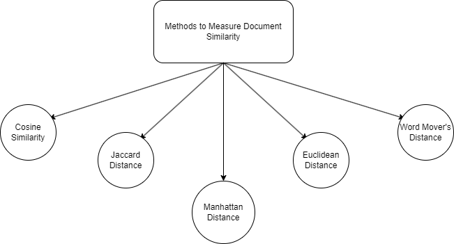
Concepts behind Document Similarity
As can be inferred from what was stated at the beginning, document similarity is is a measure of how similar two or more documents are. Now, there are multiple methods of measuring it, and we'll be having a look at a few of those methods.
-
Cosine Similarity: A widely used technique for Document Similarity in NLP, it measures the similarity between two documents by calculating the cosine of the angle between their respective vector representations by using the formula-
cos(θ) = [ (a · b) / (|a| |b|) ], where-θ = angle between the vectors,
a & b = vector representations of both the documents,
a.b = dot product of vectors a & b,
|a|,|b| = magnitude of vectors a & b respectively.
The vector representations are usually created using the term frequency-inverse document frequency (TF-IDF) method, which weighs each word in the document based on how frequently it appears in the document and inversely proportional to the number of documents it appears in. It is often used as it is fast and efficient, but it should be noted that the length of the document has some bearing on the cosine score as well- as longer documents tend to have a lower cosine similarity score.
-
Jaccard Coefficient: It calculates the similarity between two documents by dividing the number of common words between two documents by the sum total of the number of words in both documents. In simpler terms, it is the number of elements in the intersection of both documents divided by the union. It is easy to understand and implement, however just like cosine similarity, it can be affected by the size of the documents- as the larger the size becomes, the lower the score gets.
-
Manhattan Distance: Named after the pathways in Manhattan where the streets are straight and intersect at right angles, this method is used to calculate the similarity between two documents based on their vector representations, by summing the absolute values of the differences between the values at their respective coordinates.
Let's say that two documents were encoded as vectors (x1,y1,z1) & (x2,y2,z2). In that case, Manhattan Distance = |x1-x2|+|y1-y2|+|z1-z2| i.e. sum of absolute values of differences of values in corresponding axes.
Contrary to the previous methods, Manhattan Distance is unaffected by the length of the documents. However, it may not be as accurate as other methods.
-
Euclidean Distance: A measure of the distance between two points in an n- dimensional space, it is used to calculate the similarity between two documents, using their vector representations The vector representations are created using the TF-IDF vectorizarion method, similar to the cosine similarity metric.
-
Word Mover's Distance: An advanced technique for measuring Document Similarity, it measures the dissimilarity between two documents by calculating the minimum distance between the embedded words in one document and the embedded words in the other document.
Word embeddings are real-valued vectors that encodes the meaning of the words in such a way that words that are closer in the vector space are similar in meaning.
It can capture the semantic meaning of words in documents. However, it can be computationally expensive,especially for larger documents.
Now that we have a basic understanding of these methods, we shall be trying to implement them in Python.
Implementation
Cosine Similarity
First we'll be trying a naive approach to the same, using elementary libraries.
We'll first take two input documents, tokenize them and then convert them to a vector form in such a way that it is easily understood. After that, we shall find the value of the cosine similarity by dividing the dot product of the vectors by the products of their magnitudes.
import math

# sample documents
document1 = "The sun in the sky is bright."
document2 = "We can see the bright sun in the sky."

# split the documents into tokens
tokens1 = document1.split()
tokens2 = document2.split()

# create a set of unique tokens
unique_tokens = set(tokens1 + tokens2)

# create dictionaries to store the token counts for each document
count1 = dict.fromkeys(unique_tokens, 0)
count2 = dict.fromkeys(unique_tokens, 0)

# count the number of occurrences of each token in each document
for token in tokens1:
    count1[token] += 1
for token in tokens2:
    count2[token] += 1

# calculate the dot product of the token count vectors
dot_product = 0
for token in unique_tokens:
    dot_product += count1[token] * count2[token]

# calculate the magnitude of each token count vector
magnitude1 = math.sqrt(sum(count1[token] ** 2 for token in unique_tokens))
magnitude2 = math.sqrt(sum(count2[token] ** 2 for token in unique_tokens))

# calculate the cosine similarity
cosine_similarities = dot_product / (magnitude1 * magnitude2)

# print the result
print(cosine_similarities)
Running the above script returns a result of 0.4558423058385518, indicating that the two documents are somewhat similar.
Let's have a look at the proper implementation of Cosine Similarity.
# sample documents
document1 = "The sun in the sky is bright."
document2 = "We can see the bright sun in the sky."

from sklearn.feature_extraction.text import TfidfVectorizer
from sklearn.metrics.pairwise import cosine_similarity

# sample documents
doc1 = "The sun in the sky is bright."
doc2 = "We can see the bright sun in the sky."

# create TF-IDF vectorizer
tfidf_vectorizer = TfidfVectorizer()

# fit and transform the documents
tfidf_matrix = tfidf_vectorizer.fit_transform([doc1, doc2])

# compute cosine similarity between doc1 and doc2
cosine_sim = cosine_similarity(tfidf_matrix[0], tfidf_matrix[1])[0][0]
print("Cosine similarity between doc1 and doc2:", cosine_sim)
Output-

It should be noted that although the input documents being passed to both methods were the same, the proper method returns a better cosine similarity that the naive method.
Jaccard Distance
For this, we shall first define a preprocessor function, then the function to calculate the distance. It should be kept in mind that since this is a dissimilarity measure, the lesser the distance the more the similarity.
import re
import nltk
from nltk.tokenize import word_tokenize
from nltk.corpus import stopwords

#define function for data cleaning
def preprocess(text):
    text = re.sub(r'[^\w\s]', '', text)  # remove punctuation
    tokens = word_tokenize(text.lower())  # tokenize and convert to lowercase
    tokens = [token for token in tokens if token not in stopwords.words('english')]  # remove stop words
    return set(tokens)  # return set of unique tokens

#function for preprocessing data
def jaccard_distance(set1, set2):
    set1=preprocess(set1)
    set2=preprocess(set2)
    intersection = set1.intersection(set2)
    union = set1.union(set2)
    return 1 - len(intersection) / len(union)

#testing
doc1 = "The sun in the sky is bright."
doc2 = "We can see the bright sun in the sky."
distance = jaccard_distance(doc1, doc2)
print(distance)
The above code returns an output of 0.25, indicating that the two documents are quite similar.
Manhattan and Euclidean Distances
We shall present two approaches to both, namely- a naive and a proper implementation of each. Both are implemented together as they are similar in nature.
Naive Implementation
We first tokenize the two documents and create vectors from the same. Considering that the lengths of the vectors may differ, we pad the length of the smaller vector with additional 0's and then we move with implementing the formulae of manhattan and euclidean distances. Since distances are a dissimilarity measure, the lesser the distance the more the similarity.
#manhattan and euclidean distance
import numpy as np

# sample documents
doc1 = "The sun in the sky is bright."
doc2 = "We can see the bright sun in the sky."

# tokenize the documents
tokens1 = doc1.lower().split()
tokens2 = doc2.lower().split()

# create the word frequency vectors for the documents
vector1 = np.zeros(len(tokens1))
vector2 = np.zeros(len(tokens2))

for i in range(len(tokens1)):
   vector1[i] = tokens1.count(tokens1[i])

for i in range(len(tokens2)):
   vector2[i] = tokens2.count(tokens2[i])

#padding
if len(vector1) < len(vector2):
   for x in range((len(vector2) - len(vector1))):
       vector1=np.append(vector1,0)
else:
   for x in range((len(vector1) - len(vector2))):
       vector2=np.append(vector2,0)

# calculate the Manhattan distance
manhattan_distance = np.sum(np.abs(vector1 - vector2))

# calculate the Euclidean distance
euclidean_distance = np.sqrt(np.sum((vector1 - vector2)**2))

# print the result
print("Manhattan distance:", manhattan_distance)
print("Euclidean distance:", euclidean_distance)
After running this code, the outout comes out to be this.
Manhattan distance: 4.0
Euclidean distance: 2.449489742783178
Since the distance is quite less, they are similar.
Proper Implementation of Manhattan and Euclidean distances
from scipy.spatial.distance import cityblock, euclidean
# sample documents
string1 = "The sun in the sky is bright."
string2 = "We can see the bright sun in the sky."

# Convert input strings to lists of words
words1 = string1.split()
words2 = string2.split()

# Compute the maximum length of the two lists of words
max_length = max(len(words1), len(words2))

# Pad the lists of words with zeros to ensure they have the same length
words1 = words1 + [''] * (max_length - len(words1))
words2 = words2 + [''] * (max_length - len(words2))

# Compute bag-of-words representations for each string
bow1 = {word: words1.count(word) for word in words1}
bow2 = {word: words2.count(word) for word in words2}

# Compute Manhattan distance between the two bag-of-words vectors
manhattan_distance = cityblock(list(bow1.values()), list(bow2.values()))

# Compute Euclidean distance between the two bag-of-words vectors
euclidean_distance = euclidean(list(bow1.values()), list(bow2.values()))

# Print the results
print("Manhattan distance:", manhattan_distance)
print("Euclidean distance:", euclidean_distance)
Output-
Manhattan distance: 2
Euclidean distance: 1.4142135623730951
As was noticed before, the similarity for proper methods is observed s higher than the naively implemented ones.
Word Mover's Distance
We first tokenize the input strings into lists of words using the word_tokenize function from the nltk library. We then load a pre-trained Word2Vec model using the KeyedVectors.load_word2vec_format function from the gensim library. The wmdistance function from the KeyedVectors object is then used to compute the Word Mover's Distance between the two lists of words.
from gensim.models import Word2Vec
from gensim.models import KeyedVectors
from nltk import word_tokenize
import numpy as np

# sample documents
string1 = "The sun in the sky is bright."
string2 = "We can see the bright sun in the sky."
# Tokenize the input strings into lists of words
words1 = word_tokenize(string1)
words2 = word_tokenize(string2)

# Load a pre-trained Word2Vec model, mention the path in the model_path variable
model_path = 'path/to/GoogleNews-vectors-negative300.bin.gz'
model = KeyedVectors.load_word2vec_format(model_path, binary=True)

# Compute the Word Mover's Distance between the two lists of words
wmd = word_vectors.wmdistance(words1, words2)

# Print the result
print("Word Mover's Distance:", wmd)
Different Embeddings for Word Mover's Distance-
Other than Word2Vec, there are a few other models as well which can be loaded. A few examples are-
- BERT: Bidirectional Encoder Representations from Transformers (BERT) is a pre-trained language model that can be fine-tuned for a variety of NLP tasks, including document similarity. It learns contextualized embeddings that capture the meaning of the text in a more nuanced way than traditional embeddings.
- Doc2Vec: It is a neural network-based method that learns document embeddings by considering the context of the words in the document. It learns a vector representation of the document that is optimized to predict the words in the document.
- Universal Sentence Encoder(USE): The Universal Sentence Encoder model encodes textual data into high dimensional vectors known as embeddings which are numerical representations of the textual data. It specifically targets transfer learning to other NLP tasks, such as text classification and document similarity.
Do note that the model being loaded is quite large, around 3 GB in size. Also, this method would be computationally expensive as well. Hence, use of this method - which yields accurate results should however be done with the consideration of the costs involved.
Conclusion
To conclude, Document Similarity Classification is a crucial application of NLP having multiple use cases across the board and it can be implemented in multiple manners using, as follows.
Approaches Using NLP techniques
* **Cosine Similarity:** Uses the formula for the cosine of the angle between two vectors. It is fast and efficient, but scores are affected by the size of the documents.
-
Manhattan Distance/ Euclidean distance: Manhattan Distance is given by the sum of the absolute values of differences between elements at corresponding locations, while Euclidean Distance is given by the sum of squares of the absolute values of differences between elements at corresponding locations. They are robust to the size of the document, but not very efficient.
-
Jaccard Coefficient: Given by the size of the set containing words which are common to both documents divided by the length of the set containing the union of words in both documents. It is easy to understand and implement but it's limitations are similar to that of cosine similarity.
Approaches Using Deep Learning Methods
**Word Mover's Distance:** It measures the dissimilarity between two documents by calculating the minimum distance between the embedded words in one document and the embedded words in the other document, using pretrained models. It can capture the semantic meaning of the text but is computationally expensive. The use of embeddings (eg. Word2Vec, Doc2Vec) & transformers (e.g. BERT) as mentioned before makes it a **deep learning** approach towards determining similarity of documents.
In the end, each method has it's own merits and demerits, and the choice of method for a document similarity task depends on the type of the task itself.