Sentiment analysis with NLP

Introduction

In some of the previous articles, we discussed the various tasks that were done prior to training a NLP model. Now, we shall be discussing an important use case for those tasks, and by extension NLP itself, known as 'Sentiment Analysis'.

Sentiment Analysis is the method of locating and extracting subjective information from text data. It entails determining whether the emotional bias of a text is positive, negative, or neutral by looking at its contents. This has various use cases, including but not limited to-

1. Gauging public opinion towards events, policies, news etc.
2. Feedback analysis of products and services
3. Identifying customer opinions towards products, brands and trends in market research

All in all, it is a very useful application of NLP with use cases in multiple avenues, and this article shall aim to serve as a beginner's guide on Sentiment Analysis with NLP, implemented using Python.

Overview of the Process

From a bird's eye view. the overall process involved in sentiment analysis is actually quite similar to building a classification model on tabular data, as can be seen from this flowchart. The steps involved are-

• Data Gathering & Preprocessing-
  In this phase, we gather the data from various sources and assess its quality to make it more suitable for use by eliminating un-needed entities. Examples of a task falling under this phase would be removal of punctuation, special characters, stop words (if deemed necessary) and standardizing the case.
• Feature Extraction-
  Before using the data, we need to extract features out of them. This is done by using either a Bag-Of-Words model or a TF-IDF vectorizer model, among others.
• Classification-
  The final step is to classify the text data into positive, negative, or neutral sentiment using a classification algorithm in Machine Learning, examples being Logistic Regression ( for binary classification e.g. "Yes/No"), Decision Tree, Random Forest, Naive Bayes among others. In case there is no labeling on the data to be used for training the model, unsupervised approaches may be used as well. Once a proper model is obtained from the data, it can be exported for deployment.

Let's understand the process by going through it's implementation in Python.

Naive Implementation

We'll be first implementing a naive approach to sentiment analysis for a thorough understanding of the topic.

One simple algorithm would be to-

• Define two lists of words - one containing words carrying positive sentiments and the other list containing words carrying negative sentiments.
• Iterate through the text being provided and maintain two variables, initialized as zero. The first would be incremented if a match with the positive word list is found, and the other would be incremented if there is a match eith the negative word list.
• If number of positive words> number of negative words, the sentiment is "positive". Else if number of positive words = number of negative words, it is "neutral". Otherwise, it is "negative".

However, this algorithm has it's drawbacks. For example, it doesn't take into account how clean the data is, which may end up giving false results. Other than that, defining the positive word list and the negative word list manually is also a hard task, considering that the type of words being used may vary from problem to problem and that a lot of relevant words need to be included in the lists, doing which takes a lot of time and energy.

Keeping this in mind, we shall move to the next naive implementation. Before that, let's have a look at the flow chart once again.

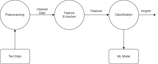
Here, we can see three stages to the entire thing, the first being preprocessing, then feature extraction and then finally, modeling. Keeping this in mind, we can split the entire script into 3 major sections - Preprocessing, Feature Extractions and Classification. Let's have a look at them one by one.

Preprocessing

#import necessary libraries
import nltk
from nltk.corpus import stopwords
from nltk.tokenize import word_tokenize
from string import punctuation
import re

STOPWORDS = set(stopwords.words('english'))

def lowercase(text):
    lowercase_chars = [char.lower() if char.isalpha()  else " " for char in text]
    return "".join(lowercase_chars)

def preprocess(text):
    text = lowercase(text)
    tokens = word_tokenize(text)
    tokens = [word for word in tokens if word not in STOPWORDS]
    text = "  ".join(tokens)
    return text

This section has two functions - lowercase , which is used in the second function i.e. preprocess. the lowercase function takes a string potentially containing all kinds of characters, and returns only the alphabetical characters in lower case. The main reason behind this is that numbers and other non alphabetical characters are not expected to have any predictive power in the context of Sentiment Analysis.

The preprocess function converts the text into lowercase by calling the precious function, tokenizes the text and removes stop words, if any. After that, the preprocessed text is returned.

Feature Extraction

from sklearn.feature_extraction.text import CountVectorizer
from sklearn.naive_bayes import MultinomialNB
def extract_features(text):
    vectorizer = CountVectorizer()
    features = vectorizer.fit_transform([text])
    return features

In this section, we convert the data into vectors which can be understood ny the subsequent ML model.

Classification

def train_classification_model(clf, text, assigned_label):
   text1= preprocess(text)
   features = extract_features(text1)
   features
   clf.fit(features, [assigned_label])
   return clf

def test_model(clf, test):
   return clf.predict(extract_features(preprocess(test)))
  

This section contains the definitions of two functions, one for training an ML model and one for testing said ML model. As this is a naive approach, we shall be using unstructured data and the architecture of these functions is tailored according to it.

In the first function which takes three parameters (model, text data and training label), the text data is passed to the preprocess function and then features are extracted from the returned value, which serve as part of a training record to the ML model, alongwith a pre specified class label. After this, the fitted ML model is then returned.

This function may be called multiple times so as to fit multiple strings and their corresponding class labels to the specified ML model.

The test_model function is then used to get the predictions of the fitted model on being passed a raw string containing a test record.

We shall now be training and testing a Naive Bayes model using these functions.

clf=MultinomialNB()
train_classification_model(clf, "I love this movie! The acting was superb and the storyline was captivating.", 'Positive')
train_classification_model(clf, "I hated the movie, the acting was bad and the storyline was boring.", 'Negative')
train_classification_model(clf, "The movie was okay, average in terms of acting and story.", 'Neutral')

test_model(clf, "The movie was average  in terms of everything. Could be better")

Output-

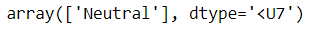
On understanding the code, it can be seen that the Naive Bayes model was passed three training records and one testing record. As can be expected, the sentiment of the passed record comes out to be neutral.

Approach Analysis -

1. Simple, easy to understand
2. Suitable for passing records to a model one by one, unsuitable for scenarios where the number of records is large. Hence, non scalable.
3. This approach only works when the number of tokens generated by a test record is same as the number of tokens generated by the text data of a corresponding training record. For example, if we try to pass "I liked the movie, it was good" to the test_model function, we won't be able to get an output. Instead, this error is returned.

It is so because the number of tokens generated by this test record is not the same as the number of tokens generated by the corresponding training record. These disadvantages warrant the need for a better, more scalable method which is robust to such problems.

Implementation using NLTK

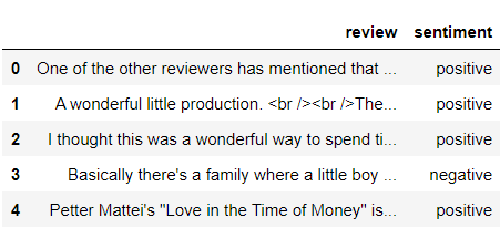
For this, we shall be using the IMDB movie reviews dataset. This dataset contains 50,000 data points, half of them having a positive sentiment and the other half having a negative sentiment.

import numpy as np
import pandas as pd
df = pd.read_csv("IMDB Dataset.csv")
df.head()

Output -

Preprocessing

Moving on, the initial phase will be quite similar to the previous approach where we write a function to preprocess the data. For the sake of completeness however, stemming is also included in said function.

import nltk
from nltk.corpus import stopwords
from nltk.tokenize import word_tokenize
from string import punctuation
from nltk.stem import *
import re

STOPWORDS = set(stopwords.words('english'))

def lowercase(text):
    lowercase_chars = [char.lower() if char.isalpha()  else " " for char in text]
    return "".join(lowercase_chars)

def preprocess(text):
    cleaner = re.compile('<.*?>')
    text = re.sub(cleaner, '', text)
    text = lowercase(text)
    text= ' '.join([PorterStemmer().stem(word) for word in text.split()])
    tokens = word_tokenize(text)
    tokens = [word for word in tokens if word not in STOPWORDS]
    text = "  ".join(tokens)
    return text

df['review']=df['review'].apply(lambda x: preprocess(x))
df.head()

The preprocess(text) function now removes any stray tags as well as performs stemming on the words of the text apart from it's usual functions i.e. converison of words to lower case, tokenization and stopword removal.

Feature Extraction

Now we move on to the second phase, where we extract features from the data. For the purposes of this article, we shall be using the tf-idf vectorizer.

When we talk about the TF-IDF vectorizer (TF-IDF being an acronym of Term Frequency-Inverse Document Frequency), it is a technique used to represent text as numerical entities, where it's importance is given by how frequently it appears in the entire corpus (hence the use of the phrase "term frequency") and how important is it to the entire document corpus(hence "inverse document frequency"). The reason behind the preference of TF-IDF vectorizer over other methods like Bag-Of-Words is that it is more robust to stopwords and noise data and hence can give better results compared to BOW.

Now, we will need to split the data into test and train datasets. We shall be taking a 4:1 ratio for train and test datasets for the sake of simplicity.

train_reviews,train_sentiments=df.review[:40000],df.sentiment[:40000]
test_reviews,test_sentiments=df.review[40000:],df.sentiment[40000:]

Using TF-IDF vectorizer, we have-

from sklearn.feature_extraction.text import TfidfVectorizer
tv=TfidfVectorizer(min_df=0,max_df=1,use_idf=True,ngram_range=(1,3))
tv_train_reviews=tv.fit_transform(train_reviews)
tv_test_reviews=tv.transform(test_reviews)

Model building and testing:

We shall now move towards the final portion i.e. model building and testing. Since this is a binary classification problem, we shall use Logistic Regression.

lr=LogisticRegression(random_state=100)
#Fitting the model for TFIDF
lr_tv=lr.fit(tv_train_reviews,train_sentiments)
test_sentiments_pred = lr_tv.predict(tv_test_reviews)

target_names = ['positive','negative'] # target values

# Print classification report after a train/test split:
print(confusion_matrix(test_sentiments, test_sentiments_pred))
print(classification_report(test_sentiments, test_sentiments_pred , target_names=target_names))

The lr.fit() method here is used to 'train' the model on the given data. Basically, the model is fed with the independent and dependent constituents of the training data. With each record being passed, the model adjusts its internal parameters to minimize the difference between its predicted output and the true output by a process called gradient descent.

In the context of logistic regression, it would mean plugging the data into the sigmoid function to generate a value between 0 to 1 which would determine the predicted output label for a certain record.

The lr.predict() method then uses the model prepared by the lr.fit() method to predict the values for independent variables of the test data. Post that, the confusion matrix and classification report methods- taking in the true and predicted values of the dependent variable provide an understanding of the performance of the model.

The output to the previous code segment is as follows-

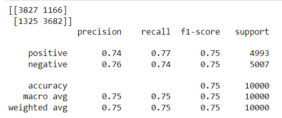
As we can see, the results are quite promising as the model has given a good result.

On comparing it with the previous approach, it can be clearly seen that it is much more suitable for a real life situation as it is-

1. More scalable, as the above model was trained on 40,000 data points.
2. Less prone to error, as the previously observed error was not encountered.

However, this model comes with it's own set of drawbacks. For example, this procedure is quite code heavy and may be difficult to explain to people who are not from a background of Machine Learning.

Keeping this in mind, we shall be moving towards the third and final approach to sentiment analysis.

Implementation using sentiment lexicons

Sentiment lexicons are pre-made dictionaries of words and the sentiment scores attached to them. These ratings, which are based on subjective evaluations, can be used to predict the sentiment of a piece of text.

We will use the AFINN-165 sentiment lexicon for the purpose of this analysis. AFINN-165 is a list of English words and their sentiment scores, ranging from -5 (most negative) to +5 (most positive). The lexicon is available for download on GitHub.

Compared to the two previous approaches, this is very straightforward. To begin, we will download the AFINN-165 sentiment lexicon and save it into a dataframe.

afinn = pd.read_csv("AFINN-165.txt", sep='\t', header=None, names=['word', 'score'], index_col='word')
afinn.head()

Output-

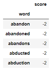
Now all that remains to be done is to define a function which iterates through a piece of text and adds the scores of all the words present in said text. If the total score is more than zero, it is positive in sentiment and else, it is negative.

def sentiment_score(text):
    words = nltk.word_tokenize(text.lower())
    score = 0
    for word in words:
        if word in afinn.index:
            score += afinn.loc[word]['score']
    return score
  
def sentiment_score(text):
    words = nltk.word_tokenize(text.lower())
    score = 0
    for word in words:
        if word in afinn.index:
            score += afinn.loc[word]['score']
    return score

def sentiment(text):
    if sentiment_score(text)>0:
        return "Positive Sentiment; Score is : "+str(sentiment_score(text))
    elif sentiment_score(text)==0:
        return "Neutral Sentiment; Score is : "+str(sentiment_score(text))
    else:
        return "Negative Sentiment; Score is : "+str(sentiment_score(text))

If we run the sentiment function on this movie review, taken from the IMDB dataset, which is -

This a fantastic movie of three prisoners who become famous. One of the actors is george clooney and I'm not a fan but this roll is not bad. Another good thing about the movie is the soundtrack (The man of constant sorrow). I recommand this movie to everybody.
Greetings
Bart

We get the following result.

These are the three methods that one could adopt in sentiment analysis tasks. Let's have a look at a few questions.

Questions to consider

With this article at OpenGenus, you must have the complete idea of Sentiment analysis with NLP.