In this article, we have covered the idea of Distance Vector in Computer Network in depth along with Routing and Distance Vector Routing protocol.

Table of contents:

1. Introduction to Routing
2. Idea of Distance Vector
3. Distance Vector Algorithms
4. Bellman-Ford algorithm
5. Implementation
6. Example
7. How it all works

Introduction to Routing

When we use the internet, the information across networks travels across the planet in small distributed pieces called packets. With the help of these packets, we receive the information that we request from the internet. Our devices then assemble these packets for us to understand the information. These packets travel across networks as per a defined protocol.

Idea of Distance Vector

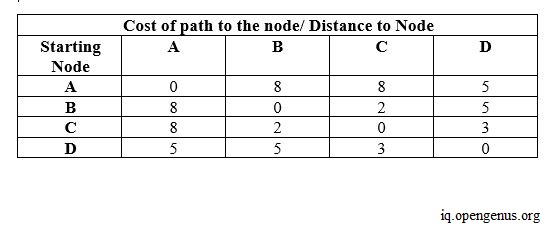
The distance vector routing protocol is one of the main protocols used for routing packets across networks. As we know, the internet is a network of networks. So, when a request is made from a network, the requested information comes in packets that travel across these networks. Usually, in these networks, the routers handle the work of directing the traffic. They handle the directions of packets. So, think of all these routers in the networks as nodes in a graph. Each router is connected to some other routers and the path through which we can reach the other router has certain costs involved with it. This path cost is shared by each router with its neighbors. Each router creates a distance vector table that contains information about the routers in the network, specifically, the cost associated to reach every router from this particular router (this is the cost of the path that the packet may take to travel). In the final distance vector table of every router, to reach the other routers, we would only choose those paths that have the least cost associated with them. Consider the example of a network shown below.

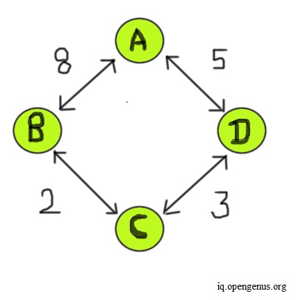
In this example, four routers form a network, and the distance to reach from one node to another has some costs involved, as shown above. When we start out building the initial distance vector table for each router, each router only fills the information it has about its neighbors. So, in this table, some routers are initially unreachable from this router. As of yet, we assume there isn't any path to reach these routers. We fill in the cost of these paths in the distance vector of this current router as infinity. Once we have finished creating the initial distance vector table for all routers, we find a path to the unreachable routers using the distance vector information of the neighbor routers from the previous iteration. We repeat this process several times, till no infinity values exist in any distance vector table. Every router updates its distance vector periodically and informs its neighbors with its new distance vector if there is any change. The image below shows the final distance vector for each node.

Counting to Infinity Problem

Sometimes there can be cases where a particular path to reach the other router may become unreachable. A router may have some trouble accessing that path. So, in the distance vector table, we set the cost of reaching such routers as infinity. The router updates its distance vector and informs its neighbors of such changes. There are cases when situations like these could lead to a problem called counting to infinity.

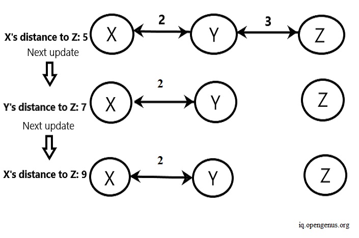
In the example shown above, router X takes the path to reach Z through Y. X to Y costs two, and Y to Z costs three, giving us a total cost to Z from X as five. Consider a scenario where the connection between router Y and router Z breaks. So all paths to router Z become invalid. In the next update, the router Y sees that router Z costs five from router X, and if we fail to update this, router Y uses the router X to reach router Z. Reaching router X costs two to router Y, and the invalid path costs router X five to reach router Z. This way, we wrongly update the path cost from router Y to router Z as seven (5+2). Now, router X sees that Z costs seven from router Y. It takes this invalid path and wrongly updates its path cost to Z as nine because it takes two to reach Y from X and Y takes seven to reach router Z. This cycle of wrong updates to the distance vectors continues.

We can see that router Z is not accessible for both router X and router Y. But, if Y doesn't inform X that the path to Z is inaccessible, and X continues to use the path to Z from Y, then it can lead to overcounting of costs and using paths that don't even exist in the network.

Solutions to Counting to Infinity

We can solve this challenge using hold-down timers, where we delay sharing distance vectors until all other routers have received the updated distance vector in case a change occurs. We can also use techniques like Split Horizon and Poison reverse. In the former, we make sure that router X never tells router Y about the cost of the path it takes to reach router Z through router Y. In the latter, we make sure that router X tells router Y that the cost of the path it takes to reach router Z through router Y has an infinity value. This way, we can avoid loops in the networks.

Distance Vector Algorithms

Usually, we use the Bellman-Ford algorithm for distance vector protocols.

Bellman-Ford algorithm

The Bellman-ford algorithm works to find the shortest path to other nodes, given a source node and a graph. It's used in distance vector and routing protocols because it takes care of all possible invalid cycles that may end up in our network structure. The algorithm begins by assigning the cost to reach the source node from the source node as zero and the cost/distance to reach the rest of the nodes in the graph from the source node as infinity. If the paths are valid and no cycle is formed, in place of infinity, we get the respective cost of the path/ distance required to reach the node from the source node. Otherwise, it stays infinity, and this helps in avoiding loops in the algorithm. We can think of the source node as the router for which we want to calculate the distance vector. Using this algorithm, we can calculate distance vectors for every router easily, without having to worry about invalid paths or cycles.

Implementation

To implement the Bellman-Ford algorithm and see how it works, follow the steps mentioned below-

• We first create a class for a graph structure. We create an attribute for its number of vertices and also create an attribute that we'll later use to store all graph edges in a list form. Within this class, we create a function to add edges into our graph, making sure to pass one parameter each for the starting vertex, ending vertex and the weight of the edge. After that, we create another function to print each edge present in the graph.
• Finally, we create our Bellman-Ford algorithm function. We include a parameter for the source node (we'll pass each node one by one as a source node to get all least cost paths). Then we create a list that initially sets the weight value of all vertices in the graph as infinity, and we set the source node's value as zero.
• Then, using a for loop, we traverse the graph V-1 times. We do this for V - 1 times because the maximum number of edges (and therefore, the length of the longest possible path) that we could take to reach from one node to another is V-1, without forming a cycle. So, for each node, when we traverse the graph for V-1 times, we make sure that we consider all possible paths. Hence, we ensure we to get to the shortest possible path for every node. Next, we compare the current weight of each path with each other, making sure to choose the smallest value.
• After we finish this loop, we once again check for a negative edge cycle. A negative edge cycle will keep on decreasing the weight of one node or more without stopping. Such cycles cause problems in networking. Hence, using a for loop, we check all edges in the graph once again. We find the negative cycle, report it using a print statement and then exit the function. In the end, we print all the edges and the weights in the graph, as per the source node given.

# create class for a graph
class Graph:

	def __init__(self, vertices):
		self.V = vertices 
		self.graph = []

	# function for adding edges to graph
	def add_edge(self, u, v, w):
		self.graph.append([u, v, w])
		
	# function to print the distance
	# of each vertex from source
	def print_vertdist(self, dist):
		print("Distance of vertex from Source")
		for i in range(self.V):
			print("{0}      {1}".format(i, dist[i]))
			# the 0 and 1 are tuple index
			# for the .format part
	
	# function to find shortest paths from source vertex
	# Can also detect negative cycles in graphs in the end
	def bellman_ford(self, src):

		# Set distance from source node to all vertex as infinity
		# set distance from source node to source node as 0
		dist = [float("Inf")] * self.V
		dist[src] = 0


		# traverse the graph V-1 times for each edge
		# to find the shortest path, without creating cycles
		
		for _ in range(self.V - 1):
                        
			# check all vertex in each edge
			# update path costs from source
			# dist[v] stores the path cost/distance from source
			for u, v, w in self.graph:
				if dist[u] != float("Inf") and dist[u] + w < dist[v]:
						dist[v] = dist[u] + w

		# check for negative weight cycle.
		# If the path's cost/distance decreases further
		# it implies a negative weight cycle

		for u, v, w in self.graph:
				if dist[u] != float("Inf") and dist[u] + w < dist[v]:
						print("Graph contains negative weight cycle")
						return
						
		# print every vertex's distance from source
		self.print_vertdist(dist)



# An example to text the above program
example_graph = Graph(5)
example_graph.add_edge(1, 2, 4)
example_graph.add_edge(1, 3, 3)
example_graph.add_edge(2, 4, 2)
example_graph.add_edge(3, 2, 5)
example_graph.add_edge(4, 3, 1)

# we pass vertex 1 as source node
example_graph.bellman_ford(1)

The above program produces the following output-

Distance of vertex from Source
0      inf
1      0
2      4
3      3
4      6

Complexity

• Time: The time complexity of the distance vector algorithm is E(V) in the worst case. This is because we traverse the graph V-1 times for every edge. This helps us to find the shortest path possible. In the best case, we have O(E) runtime, if each vertex connects to the other in a linearly fashion inside the graph.
• Space: Space complexity depends on the number of vertices in the graph. This gives a space requirement of O(V).

Example

Let’s examine the code example above to understand how the Bellman-Ford algorithm and distance vector work.

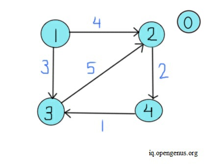
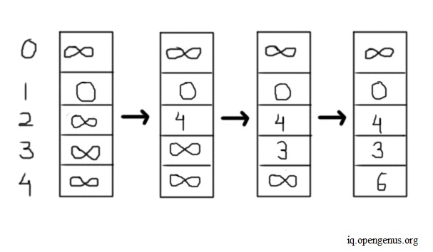
In the example, we create a graph containing five vertices. Now, we add edges one by one. We insert an edge running from vertex 1 to vertex 2, with four as weight. Then, we insert an edge from 1 to 3, weighing three, and from 2 to 4, with two as weight. Lastly, we insert two edges, from 3 to 2 and 4 to 3, having five and one as weights, respectively. Next, we call the bellman_ford function and pass vertex 1 as the source node. Initially, the algorithm sets the distance/ weight/ cost of paths from node 1 to every other node as infinity. The distance of node/vertex 1 from itself remains zero. Now, we check each edge one by one for a total of V-1 times. We check the edge running from vertex 1 to 2. The value of dist[1] is zero, and dist[1] plus a weight of four is less than dist[2]. As dist[2] is infinity, we set dist[2] as equal to four. Next, we check the edge from vertex 1 to vertex 3.

Since dist[1] is zero and zero plus the weight of three is less than dist[3] (which is infinity), we set dist[3] as equal to three. Now, we move to edge running from vertex 2 to 4. The value of dist[2] is equal to four, and four plus the weight of two is six. Since six is less than infinity, we set dist[4]'s value as six. Now, we check the edge from vertex 3 to vertex 2. The value of dist[3] is three, and three plus a weight of five equals eight. Since eight is greater than the value of dist[2], we move on to the next edge. Now, we check the edge from vertex 4 to 3. Since the value of dist[4] plus a weight of one exceeds dist[3]'s value, we move on to the next iteration. The image below shows this entire process for vertex 1's distance vector table.

After checking all edges V-1 times, we exit the current loop and go to the final loop. In the last loop, we check for negative edge cycles. There isn't any such cycle in this case, so we exit this loop. Lastly, we print the distance of each vertex from the source node.

In this example, we have taken vertex 1 as a source and only shown its distance-vector table. Likewise, each node has its distance vector, and the algorithm in protocols calculates distance-vector tables for all nodes in real-time parallelly.

How it all works

As explained in the beginning, the distance vector algorithm mainly does the following -

1. All routers inform each other about their distance vector periodically. Every router initially has information only about its neighbors in the first pass of the distance vector table.
2. Every router sends and receives the latest distance vector, from its neighboring routers.
3. In case any router's distance vector changes, it informs its neighbors accordingly.
4. The distance vector sent by each router contains the least costly path to reach every other.

Let’s see how the entire process works and how the distance vector table updates for each node in a network. For this, consider the previous example where we had four routers in a network, named A, B, C, and D, respectively.

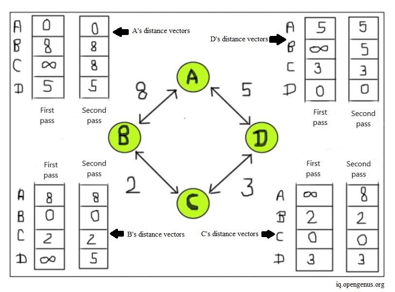
We first begin with router A's distance vector. As we can see in the image below, router A initially contains path information only about its neighboring routers. So, the cost of routers that are not its neighbors is set as infinity. In this first pass of the distance vector for router A, we have a path to reach routers B and D, but not C. Parallelly, we repeat this same process for all routers in the network.

Now we check the distance vector for router B. Router B's neighbors are router A and router C. Therefore, B's distance vector in the initial pass contains path costs to reach router A and router C. Next, we do the same check for router C. C's neighbors are router B and router D. Thus, C's distance vector initially only knows the path costs from router C to routers B and D, respectively. Lastly, we check the distance vector for router D. D's neighbors are router A and C. So, we include their path costs in router D's initial distance vector table.

Now, we move on to the second iteration. We start again with router A. Here, using distance vector tables of A's neighbors B and D from the previous iteration, we find additional paths. From the previous iteration, we see from router B's distance vector that we can reach router C from A at a cost of 10. We use B as the connecting router to reach C (here, we can call B as the intermediate hop for A to reach C). Likewise, from router D's distance vector, we can reach C from A using D as an intermediate hop. This gives us a path cost of eight. Since the path from A to D and then to C costs less than the route to C from A using B, we choose router D to reach router C from A. Now, we update router A's distance vector table. A now informs its neighbors about changes in its distance vector.

Next, we do the same for router B. Using the distance vectors of B's neighbors from previous iterations, we find that we can reach router D from B using router A or router C, at a cost of 13 and 5, respectively. Hence, we choose router C to reach router D from B and update B's distance vector. Now, we check router C's distance vector. We can reach router A from router C using router B or D, at a cost of 10 and 8, respectively. So, we choose the path using router D and update router C's distance vector.

Lastly, we check router D's distance vector. Using the information from D's neighbors and their distance vector, we have a path to reach router B from D, using router A or C. Since using C us an intermediate hop costs less to reach router B from D, we choose this path. Finally, we update router D's distance vector. This way, the distance vector algorithm finds the least-cost paths from one router to another in a network infrastructure.

With this article at OpenGenus, you must have the complete idea of Distance Vector in Computer Network.