Reading time: 40 minutes | Coding time: 10 minutes

In this article, we will see what Exploratory Data Analysis (EDA) is, what are the different steps in it, and further how to implement the same using Python.

What is Exploratory Data Analysis?

If you have just stepped into Machine Learning, you may have heard a lot of domain experts explicitly telling you to focus on the EDA phase rather than directly jumping to building the model and making predictions. And, in fact, it's true since most of the top scores, which we see in a Kaggle or some other competition, have performed some rigorous data analysis.

Exploratory data analysis is a set of analysis which is used to generate summary from data sets and present the main points in visual form.

The steps of performing Exploratory Data Analysis are:

• Loading data and identifying Target & Feature variables
• Univariate Analysis
• Bivariate Analysis
• Missing Value Treatment
• Outlier Detection and Treatment
• Feature Engineering

1. Loading data and identifying Target & Feature variables

In this step, the data is loaded generally loaded in the form of a data-frame, and independent variables (features) and dependent variable (target) are identified. Also, the data-type of each variable is identified since it further helps in analyzing the patterns and analysis to be carried out.

2. Univariate Analysis

In this step, only one variable is analyzed at a time. For instance, if we have a continuous variable, we are interested in measures of central tendency (mean, median, and mode), while for the discrete variables (categorical), we prefer frequency table. Histograms & Boxplots are often used for continuous variables and bar-chart for discrete variables.

3. Bivariate Analysis

In this step, two variables are analyzed at a time. There exists 3 possibilities- continuous & continuous, categorical & categorical and continuous & categorical. For continuous & continuous, a scatter plot is drawn and correlation between the 2 varibales is observed. For categorical & categorical, two-way table or stacked column charts are used for analyzing. In case of continuous & categorical, a box-plot can be drawn for each category type of categorical variable or further we can perform Z-test/T-test or ANOVA.

4. Missing Value Treatment

There exists a possibility that several values might be missing from the dataset. So, we have to fix them since most of the Machine Learning algorithms which we use do not take care of missing values automatically. The first possibility is to drop/remove the rows having missing value, but this method is not intuitive since we are losing some vital information. Instead, we prefer to impute the missing values using mean/median (continuous variables) or mode (categorical variables).

5. Outlier Detection and Treatment

There exists a possibility that a particular observation might be far away from the normal pattern/trend of existing values; such a value is termed as an Outlier.
If we are analyzing the salaries of different people in an organization, then the salary of the CEO can be regarded as an outlier, since it is enormous when compared with other people. Often outliers occur due to data-entry errors. It depends on the use-case and business understanding, whether you want to remove the outlier or keep it or transform it (say using log-value).

Outliers can be detected using a box-plot. If the value is less than Q1 – 1.5×IQR or more than Q3 + 1.5×IQR, then it referred to as an outlier. For multivariate outliers, we have to look at the distribution in multi-dimensions.

6. Feature Engineering

This is the most important step in EDA, and there are no fixed guidelines for this. So, an individual has to use his/her domain knowledge and creative thinking. Feature engineering means to create new features from the existing ones to extract meaning information from the existing data.

This can be further categorized into two types- Feature transformation & Feature creation. In the first, techniques like taking logarithmic (beneficial for skewed data), taking square/cube root, or making bins (making age-groups like kids, teenagers, adults, old). New features can also be derived like extracting date, month, year from a date, or identifying the age of individual using his/her date of birth or calculating savings by subtracting expenses from the total income and many more.

Implementation in Python

I have used dataset from this practice contest. https://datahack.analyticsvidhya.com/contest/practice-problem-loan-prediction-iii/

Importing necessary libraries

import numpy as np
import pandas as pd
import seaborn as sns
import matplotlib.pyplot as plt
import sklearn

Loading the data into dataframe

df = pd.read_csv('train.csv')
test = pd.read_csv('test.csv')
ids=test['Loan_ID']
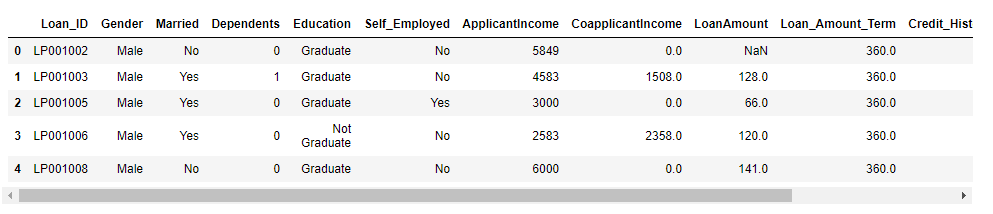
df.head()

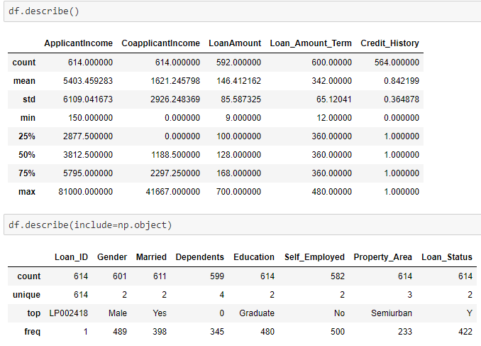
Descriptive statistics of the data
Used include=np.object for discrete variables

df.describe()
df.describe(include=np.object)

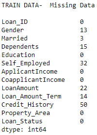
Checking for missing data

print('TRAIN DATA- ',end=' ')
if(any(df.isnull().any())):
    print('Missing Data\n')
    print(df.isnull().sum())
else:
    print('NO missing data')

Treating missing data by imputing with median (continuous) & mode (discrete variables)

df['Gender'] = df['Gender'].fillna(df['Gender'].mode()[0])
df['Married'] = df['Married'].fillna(df['Married'].mode()[0])
df['Dependents'] = df['Dependents'].fillna(df['Dependents'].mode()[0])
df['Self_Employed'] = df['Self_Employed'].fillna(df['Self_Employed'].mode()[0])
df['Credit_History'] = df['Credit_History'].fillna(df['Credit_History'].mode()[0])
df['LoanAmount'] = df['LoanAmount'].fillna(df['LoanAmount'].median())
df['Loan_Amount_Term'] = df['Loan_Amount_Term'].fillna(df['LoanAmount'].mode()[0])

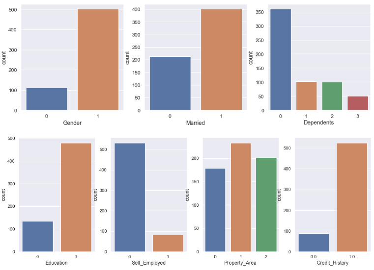
Univariate Analysis of Categorical Features

plt.figure(figsize=(16,5))

sns.set(font_scale=1.2)
plt.subplot(131)
sns.countplot(df['Gender'])

plt.subplot(132)
sns.countplot(df['Married'])

plt.subplot(133)
sns.countplot(df['Dependents'])

plt.figure(figsize=(18,6))
plt.subplot(141)
sns.countplot(df['Education'])

plt.subplot(142)
sns.countplot(df['Self_Employed'])

plt.subplot(143)
sns.countplot(df['Property_Area'])

plt.subplot(144)
sns.countplot(df['Credit_History'])

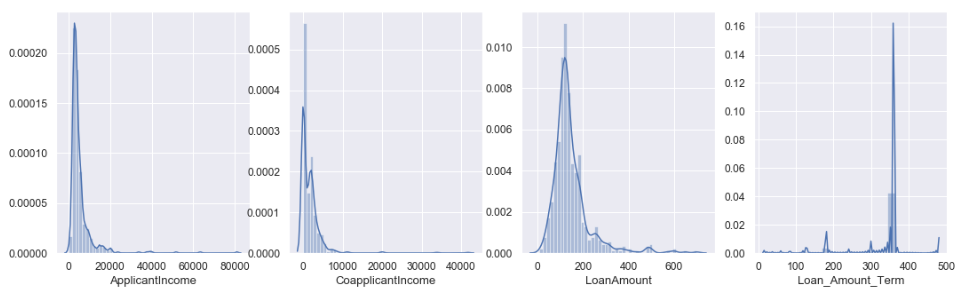
Univariate Analysis of Continuous Features

sns.set(font_scale=1.1)
plt.figure(figsize=(18,5))


plt.subplot(141)
sns.distplot(df['ApplicantIncome'])

plt.subplot(142)
sns.distplot(df['CoapplicantIncome'])

plt.subplot(143)
sns.distplot(df['LoanAmount'])

plt.subplot(144)
sns.distplot(df['Loan_Amount_Term'])

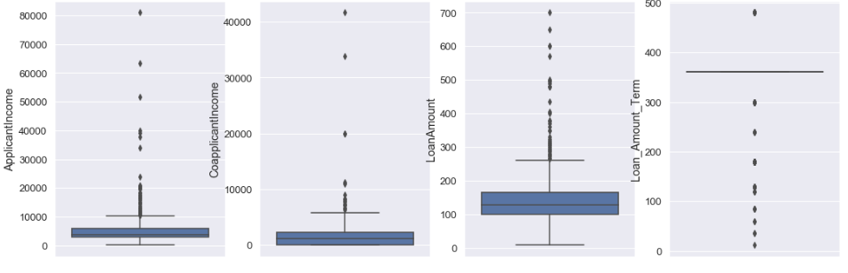
Boxplot

sns.set(font_scale=1.2)
plt.figure(figsize=(18,6))

plt.subplot(141)
sns.boxplot(y=df['ApplicantIncome'])

plt.subplot(142)
sns.boxplot(y=df['CoapplicantIncome'])

plt.subplot(143)
sns.boxplot(y=df['LoanAmount'])

plt.subplot(144)
sns.boxplot(y=df['Loan_Amount_Term'])

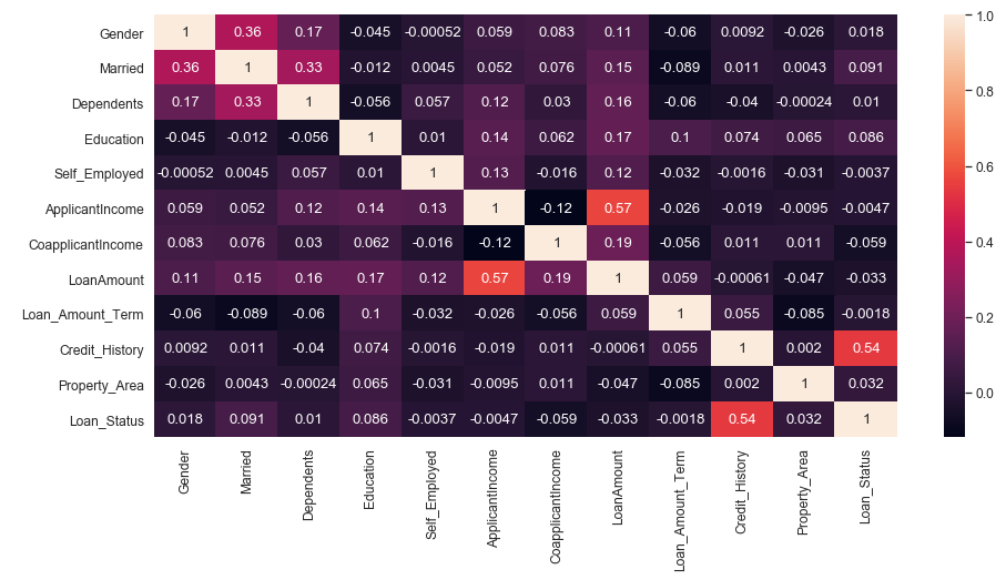
Multivariate Analysis (Bi-variate analysis can also be done using this by observing the correlation value between any 2 features)

plt.figure(figsize=(15,7))
sns.set(font_scale=1.1)
sns.heatmap(df.corr(),annot=True)

Feature Engineering by creating new features like totalincome, emi and balance income and at the same transforming total_income by using logarithmic.

df['total_income'] = np.array(df['ApplicantIncome'].tolist()) + np.array(df['CoapplicantIncome'].tolist())

df['emi']=1000*df['LoanAmount']/df['Loan_Amount_Term']

df['total_income']=np.log(df['total_income'])
df['Balance Income']=df['total_income']-(df['emi'])

Conclusion

In this post, we saw different steps of Exploratory Data Analysis and the implementation for the same in Python. The full Jupyter notebook can be accessed from here- https://github.com/akki3d76/Loan-Prediction-Problem/blob/master/LOAN%20PREDICTION.ipynb

Thank You!