Open-Source Internship opportunity by OpenGenus for programmers. Apply now.
In this article, we will learn how the hill climbing algorithm works for local searching. This algorithm is a heuristic search algorithm, a concept prominently explored in areas of Artificial Intelligence (AI). So, let us explore that and more!
Table of contents:
- What is a Heuristic Search Algorithm?
- Hill Climbing Algorithm
- Types of hill-climbing algorithms
- Simple Hill Climbing
- Steepest Ascent hill climbing
- Stochastic hill climbing
- Problems with this approach
Let us get started with Hill Climbing Algorithm.
What is a Heuristic Search Algorithm?
Where algorithms are concerned, every approach performs differently in aspects of accuracy, optimality, memory utilization, precision, speed, etc. In order to achieve perfection in some aspects, the algorithm may have to compromise on others.
A Heuristic Search Algorithm is an algorithm which prioritizes speed over optimality when looking for a solution. So, we use them in situations where we are working with time constraints and a perfectly optimal solution isn't required. A quick approximate solution can be employed. We aren't chasing perfection. We just need it to be good enough.
Hill Climbing Algorithm
Hill climbing algorithm is a local search algorithm, widely used to optimise mathematical problems. Let us see how it works:
This algorithm starts the search at a point. At every point, it checks its immediate neighbours to check which neighbour would take it the most closest to a solution. All other neighbours are ignored and their values are not stored. If at any point, the algorithm finds that none of the immediate neighbours cannot optimise the solution any further, the current point is returned as the solution.

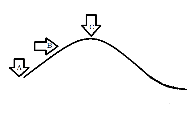
If we see this approach with an analogy to hill climbing, the algorithm begins at point A. Here, the point of highest elevation provides the most optimal solution. So, at point, the algorithm decides to take a step forward, as the height is increasing in that direction. At the next step, all neighbours are checked, which, in this simplified case, are a forward step or a backward step. Since, we need to go uphill, we take a forward step. The algorithm continues this way, taking forward steps until the peak C is reached. At point C, no further steps either forward or backward can take us any higher. So, point C is returned as the solution.
So, Hill climbing algorithm is a greedy local search algorithm in which the algorithm only keeps track of the most immediate neighbours. Once a step has been taken, you cannot backtrack by multiple steps, because the previous states are not stored in memory. At every point, the solution is generated and tested to check if it gives an optimal solution to our problem.
Types of hill-climbing algorithms
Types of hill-climbing algorithms are:
- Simple Hill Climbing
- Steepest Ascent hill climbing
- Stochastic hill climbing
We will now explore each type deeper.
- Simple Hill Climbing: This approach checks all neighbours one by one to see if any neighbour can provide a better solution to the problem. The first encountered neighbour which provides a more optimal value is chosen as the next current value.
Algorithm for Simple Hill climbing:
- Assess the current state. If it is the goal state, return success.
- If step 1 didn't return success, loop through through the current state's neighbours:
- Pick a new state and assess it:
3.1. If it is the goal state, return success and exit.
3.2. Else if it is better than the current state we had assessed, assign this new state as the current state.
3.3. Else if it is not better than the current state, then return to Step 2 and continue looping. - Exit.
- Steepest Ascent hill climbing: This approach builds up on the former, and checks all the neighbours for solutions. The neighbour which provides the best answer i.e. the steepest hill is considered to be the next current value.
Algorithm for Steepest ascent hill climbing:
- Assess the current state. If it is the goal state, return success.
- If step 1 didn't return success, we initialise a value Best_Successor.
- Now, Pick a neighbouring new state and assess it:
3.1. If the new state is the goal state, return success and exit.
3.2. Else if the new state is better than the Best_successor state, then assign this state to Best_successor.
3.3. Else if the new state is worse than the Best_Successor, discard this new state and pick another one. - Assign Current State := Best_Successor and continue looping
- Exit.
- Stochastic hill climbing: This approach selects a neighbour at random and checks it to see if it provides a better solution. Then, it is compared with the current state and depending on the differences in the values, it decides whether to examine a different neighbour or continue with the one that was just evaluated.
Problems with this approach
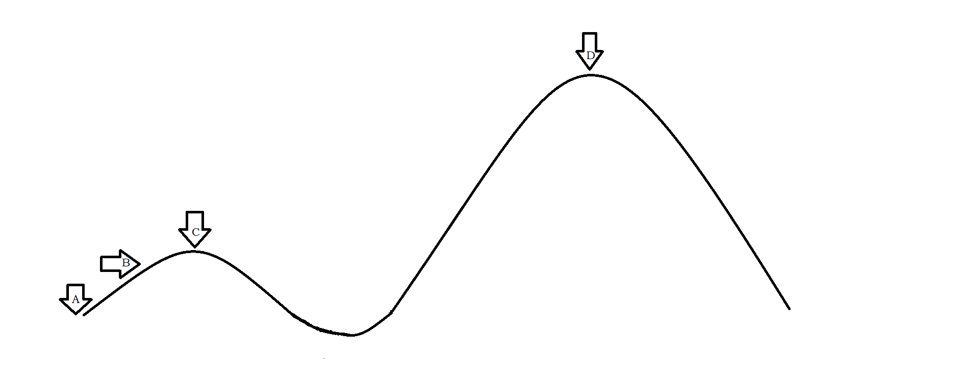
Looking at the image earlier, we see that this approach takes a very short sighted view of the problem. If we zoom out, we have the following scene

In this scenario, it is clearly visible that, while our algorithm stops at C, we do have a better solution available at point D, which cannot be reached from point A, as the algorithm stops at point C. In this case, point C is referred to as the local maximum value, while D is the global maximum.
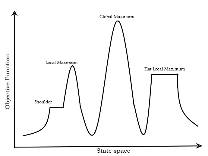
Let us now see a more detailed two-dimensional state space landscape, which sheds light on more situations in which this simple approach can fail. 
In this diagram, objective function is the function which we need to maximize/minimize in order to arrive at the optimal solution. We see that the state space landscape has a lot more variety than just crests and troughs.
-
Local Maximum is a state which is optimally better than all its neighbouring states. So, if the hill climbing algorithm arrives at this point, this value will be returned.
-
Global Maximum is the best state possible in the landscape. This is the highest point in the state space landscape.
-
Flat Global Maximum is an area where all neighbouring states are at the same elevation i.e. each solution is as optimal as the others. So, any of these points could be chosen.
-
Shoulder is a plateau region which ends with an uphill edge. In this situation, the plateau area acts like a flat region, where all points are equally suitable solutions. But we know that although the plateau ends with an uphill edge, the algorithm may not continue its search until it reaches the edge and prematurely return the shoulder region point as the solution, instead of continuing to look for higher points.
Fixing the Local Maximum Problem
Backtracking must be employed by storing the traversed states to ensure the search does not stop at a local maximum. Once a local maximum is achieved, the algorithm can backtrack to explore other paths. In this case, we have the chance to arrive at better solutions.
To avoid being stuck in a plateau/ flat local maximum
The algorithm must be modified to make sure that whenever the algorithm arrives at a plateau region, we increase the size of the step i.e. we stop checking the immediate neighbours and instead look at points some distance away from our current state. This way, we can cover the plateau region quickly and have better chances of finding the uphill edge.
Dealing with Ridges
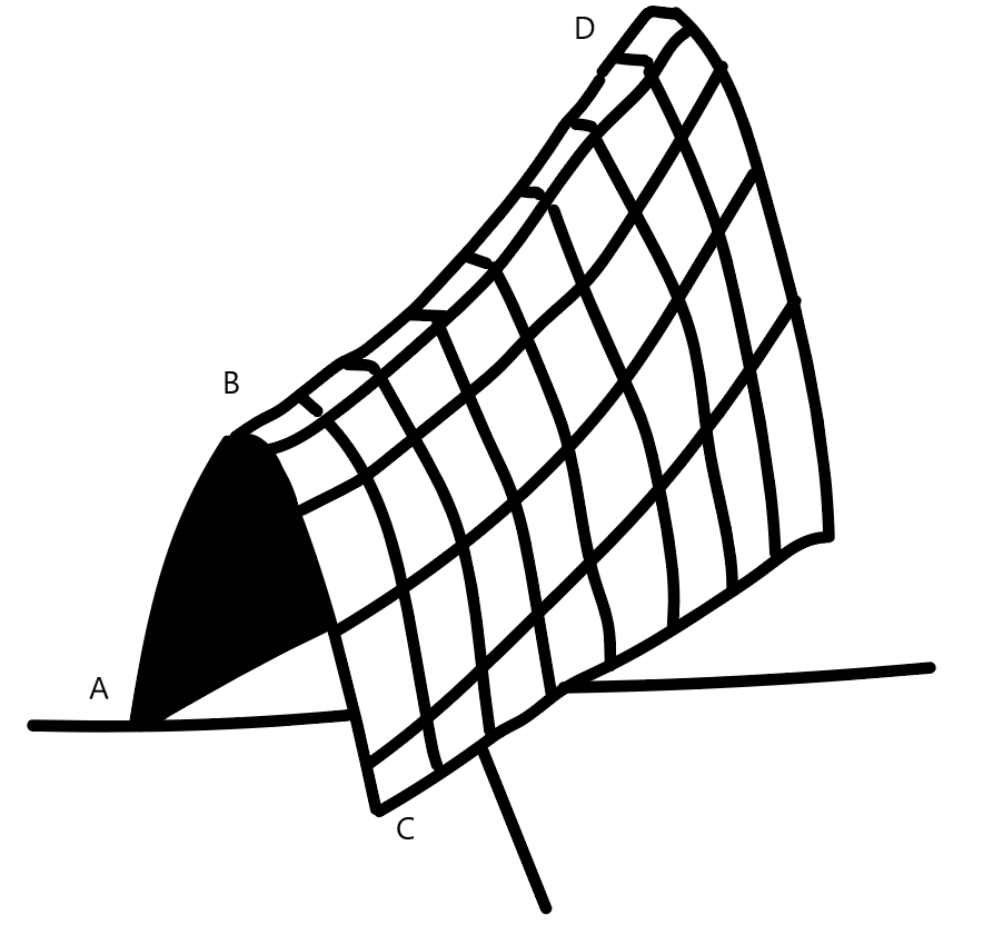
To keep the algorithm, we have only been considering a two-dimensional landscape. But in real world problems, we have situations like these:

This is called a ridge. We see that if we just consider 2-D forward and backward steps, the solution obtained will not be the most optimal. We see that starting at A, we may reach B and the algorithm stops, since any forward steps will lead to a descent. But we observe that point D has higher elevation than point B, but cannot be reached as its direction does not align doesn't align with the motion of our algorithm. The solution of this situation would be to travel in multiple directions to account for ridges.
Thus, through this article at OpenGenus, we have seen the hill climbing algorithm as well as its types. We have also explored its limitations and how they can be resolved. Keep learning!
