
Intro
Neural Collaborative Filtering(NCF) is a generalized framework to perform collaborative filtering in recommender systems using Deep Neural Networks(DNN). It uses the non-linearity, complexity as well as the ability to give optimized results of DNNs, to better understand the complex user-item interactions. This groundbreaking research was conducted by Xiangnan He, Lizi Liao, Hanwang Zhang, Liqiang Nie, Xia Hu and Tat-Seng Chua at National University of Singapore, Columbia University, Shandong University and Texas A&M University. NCF elucidates the limitations in using Matrix Factorization(MF), a simple inner product of latent features that depict user and item interactions and implicit feedback. This paper finds a solution to this by proposing a combined architecture consisting of Generalized Matrix Factorization(GMF) and Multi-layer Perceptron(MLP). Another key result is - it proves that NCF is a generalization of MF. NCF paves a way to utilize DNNs in recommender system through promising results by testing on 2 huge real world datasets - MovieLens and Pinterest.
Table of Contents
- Background
1.1 What are Recommendation Systems?
1.2 What is Collaborative Filtering?
1.3 What are the different types of Feedback? - Learning from Implicit Feedback Data & its limitations
- Matrix Factorization & its limitations
- NCF architecture
4.1 How is NCF a generalization of MF?
4.2 Generalized Matrix Factorization architecture
4.3 Multi-Layer Perceptron architecture
4.4 NeuMF architecture - Results and Discussion
5.1 Test Datasets Description
5.2 Evaluation Metrics
5.3 Parameter Setting
5.4 Performance Comparison with Baselines
5.5 Pretraining Improvement
5.7 Log Loss with Negative Sampling - Does deep learning give better recommendations?
Background
Before moving any further, let's understand all the important terms pertaining to recommendation systems, including itself!
What are Recommender Systems?
Recommender or recommendation systems are algorithms that aim to understand the customer's preferences, interest and liking in order to suggest them products that they would most likely prefer to buy. These suggestions are based on various factors of the customer's profile and/or historical data on product and customer interaction. It can simply be understood as suggesting your friend a movie based on his/her likes and dislikes. Another example is you would most likely like a dress if its of your favorite color. Nowadays, recommendation systems are utilized by top businesses to improve their sales. Some notable examples are product recommendations on Amazon based on your purchase and view history, content recommendations by Netflix based on your watch history and preferences, Tinder helps to find the best match based on the past swipes and other preferences, Instagram suggests reels based on past engagements with similar reels and content creators and many more. Such recommendation systems are built using various algorithms broadly categorized as collaborative as well as content based filtering. As NCF is a neural collaborative filtering algorithm, we will understand collaborative filtering.
What is Collaborative Filtering?
Collaborative filtering uses past user-item interactions described as a latent feature vector to predict future interactions of users in an embedding space. MF was the most commonly used algorithm to perform collaborative filtering by a performing an inner product on user-item latent vectors. We will later prove why this simple operation is not sufficient to capture the complex user-item interactions. Collaborative filtering uses feedback captured by the system to give suggestions. Hence, let's take a look at different types of feedback.
What are the different types of Feedback?
Feedback is any interaction between the user and the item that gives us significant information about the user's reaction regarding that item. It is important to note that the feedback can be either negative(dislike the item) or positive(like the item). Feedback can be of various forms - Implicit, Explicit or Hydrid.
-
Implicit feedback consists of indirect interactions of users with the item. This includes clicking items, watching videos till the end, wishlisting products, subscribing to a channel, etc. User satisfaction cannot be tracked with this feedback but it is very easy to obtain and process. There is a natural dearth of negative feedback here.
-
Explicit feedback includes direct interaction of users with the item. Liking or disliking a video, giving ratings, giving reviews, left swiping a person on Tinder, etc. are examples of the same. User satisfaction can be easily tracked as positive or negative but it is difficult to obtain and process.
-
Hydrid feedback is the combination of both Implicit and Explicit feedback. It is difficult to obtain and process. Positive and negative reviews can be captured depending on the user's interactions for that particular item. All current e-commerce websites work on Hybrid feedback for their recommendation systems.
Neural Collaborative Filtering focuses on a neural network based implementation of collaborative filtering on implicit feedback
Learning from Implicit Feedback Data & its limitations
Since, this work is based on implicit feedback, we will be delving deep into how implicit feedback data is mathematically represented, how it is utilized by mathematical models for recommendation and its challenges.
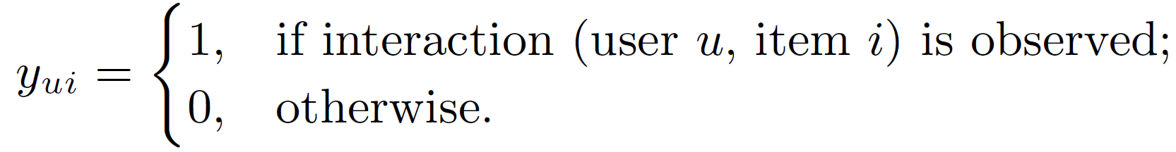
A mathematical representation of implicit data where yui is every element of the user-item interaction matrix, Y ∈ ℝMXN with M users and N items is shown in Equation 1. A value of 1 represents an interaction between user u and item i and a value of 0 shows that there hasn't been any interaction. Both values don't give any insight on whether the user ultimately liked or disliked the item as a user might interact and not like the item, and be completely unaware of the item which the user might have liked. Hence, the data collected via implicit feedback is noisy in nature and doesn't give a clear picture on the user preferences. While, these observed entries reflect a user's minimum interest in the item, there is no means of gaining a negative feedback on the item. Hence, unobserved entries are taken as missing data for the built mathematical model.
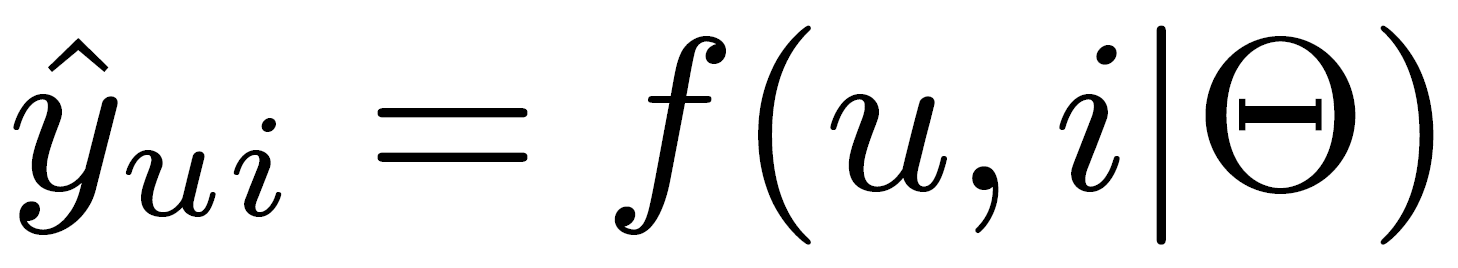
For a recommendation system, the problem can be formulated as estimation of score calculated using Equation 2 where ^yui represents the predicted score, f denotes the interaction function for calculating model parameters θ. Machine learning approaches aim to estimate parameters to optimize the objective function. This objective function can either be pointwise or pairwise loss. Pointwise loss aims to punish the predictions(^yui) that have a greater difference from the target value(yui) and hence consider unobserved entries as negative feedback. Pairwise loss is based on the idea that observed entries are ranked higher than unobserved entries and therefore the aim is to maximize the margin between observed entries and unobserved entries.
NCF aims to formulate the the interaction function fusing neural networks to estimate ^yui by taking both pointwise and pairwise losses.
Matrix Factorization & its limitations
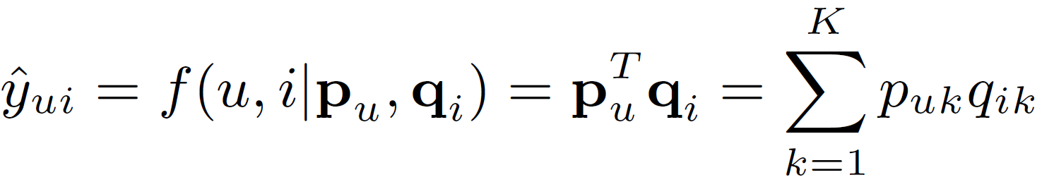
Matrix Factorization(MF) performs collaborative filtering by performing an inner product of pu and ^qi where users and items is mapped to a latent feature vector respectively as shown in Equation 3. So, the interaction function mentioned in the previous section is inner product function here.
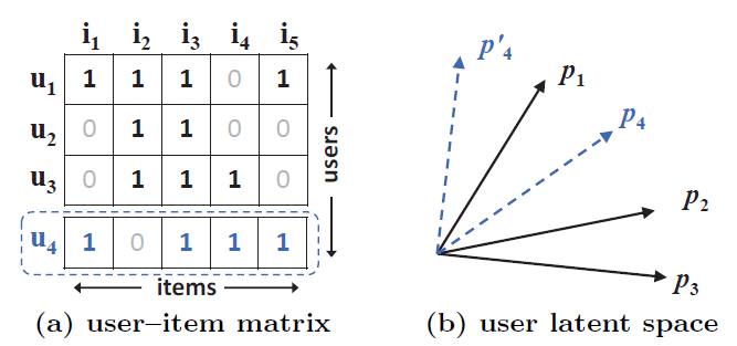
MF models the two-way interaction of user and item latent factors, assuming each dimension of the latent space is independent of each other and linearly combining them with the same weight, making it a linear model of latent vectors. This limits the expressiveness of MF making it incapable of encapsulating the complex nature of user-item interactions. An example to understand this is shown in Figure 1. Here, MF maps users and items to the same latent space, the similarity between two users can also be measured with an inner product, or equivalently, the cosine of the angle between their latent vectors considering unit length latent vectors. If we resolve the issue by choosing a higher dimensional K, it leads to overfitting hence hurting the generalization of the model.
NCF architecture
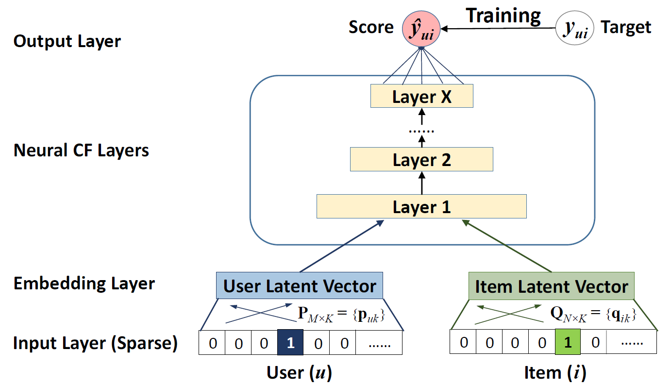
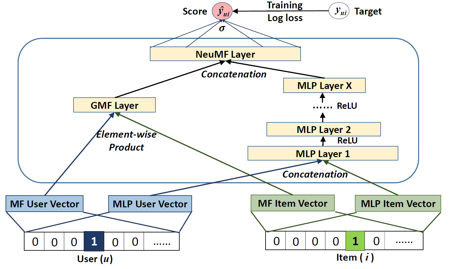
Figure 2 represents the novel NCF architecture implemented using MLP. It consists of 4 layers for performing collaborative filtering using neural networks.
-
Input Layer - The starting layer of the NCF architecture takes in one-hot encoded sparse item and user vectors as vUu and vIi. This very efficiently addresses the cold start problem of any recommender system as the input vectors used here are sparse.
-
Embedding Layer - To make the sparse layers dense, a fully connected layer works as an embedding layer. The generated item and user dense vectors can be seen as latent feature vectors that are inputted into the deep Neural CF layer.
-
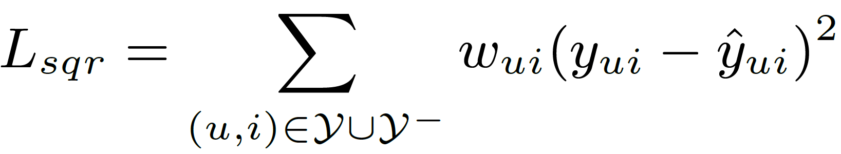
Neural CF Layer - Coming from the basic understanding of neural networks, we understand that each layer of the neural CF layers can be customized to discover certain latent structures of user-item interactions. For optimization of the objective function(shown in Equation 4), a squared loss function(shown in equation 5) is adopted.

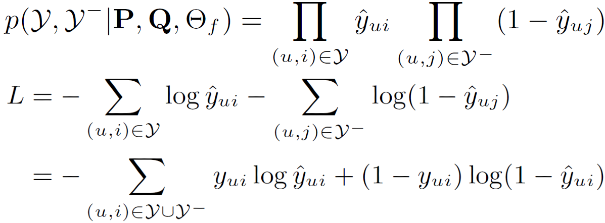
- Output Layer - The final layer, the output layer consists of predicting the target value i.e. yui as a label 1 means item i is relevant to u, and 0 otherwise. Now, the squared loss doesn't tally well with the binary target values(0 or 1 interaction values). Hence, a probabilistic approach for learning the pointwise loss is taken as a logarithmic function(sigmoid or probit function) of the likelihood function p shown in Equation 6. The obtained loss function is in the form of Log loss. The problem has now become a binary classification problem. For the negative instances Y-, we uniformly sample them from unobserved interactions in each iteration and control the sampling ratio w.r.t. the number of observed interactions. Optimizer used is Stochastic Gradient Descent Approach (SGD).
How is NCF a generalization of MF?
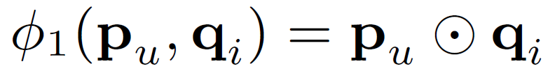
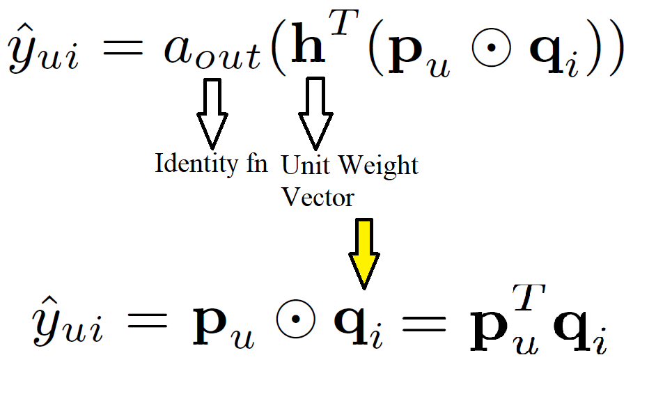
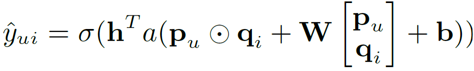
Since MF is the widely accepted algorithm for recommendation, proving that NCF is the general case of MF allows NCF to cover a large family of factorization models. As the one-hot encoded item and user vectors are embedded to give dense vectors, these work similar to latent feature vectors used in MF. Let the user latent vector pu be PTvUu and item latent vector qi be QTvIi. We define the mapping function 𝚽1 of the first neural CF layer as shown in Equation 7. The final prediction is shown in Equation 8. Intuitively, if we use an identity function for aout and h as a unit weight vector, then it resembled the MF equation for target prediction. Hence proving that MF is a special case of NCF.
Generalized Matrix Factorization architecture
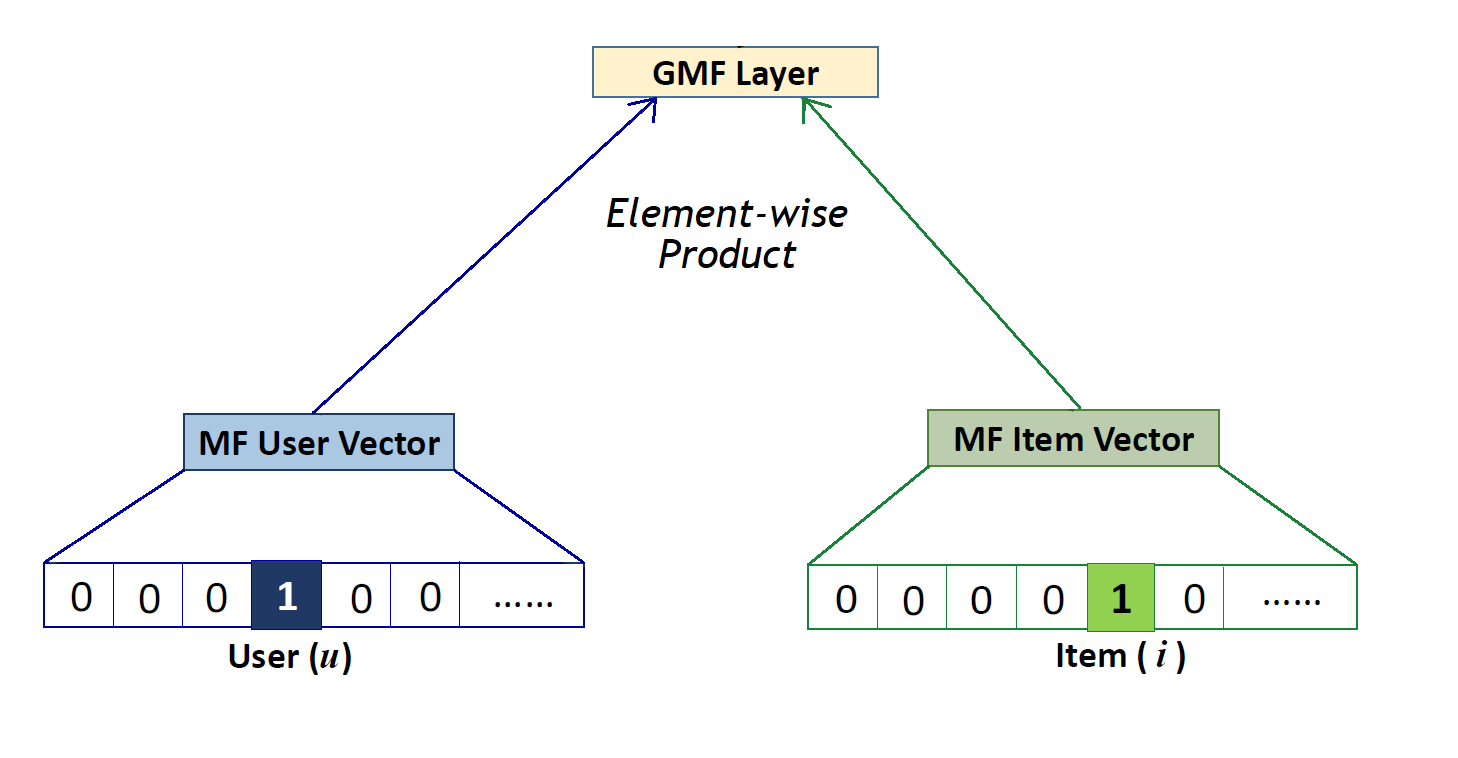
Having proven that MF is a special case of NCF, we can obtain generalized and extended MF from NCF prediction formula(top formula of Equation 8). h the weight vector is learnt from data instead of fixing it as a constant, the resultant model will be a variant of MF that looks at varying importances of latent features. On the other hand, if aout the activation function of final layer is taken as a non-linear function, the recommender will have higher expressiveness compared to a linear model. For creating the Generalized Matrix Factorization(GMF) (Figure 3) section, a generalized version of MF using a sigmoid activation function and learning weights from data is implemented.
Multi-Layer Perceptron architecture
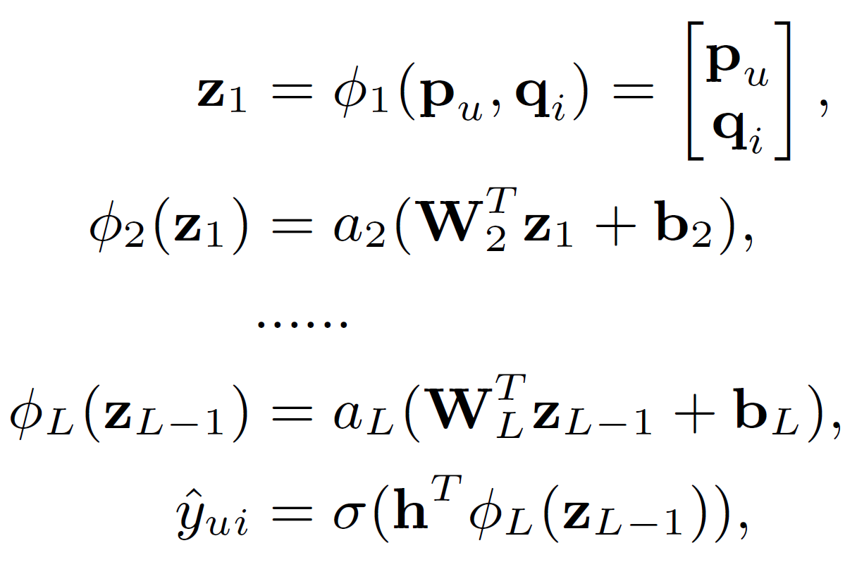
As we have already discussed that linear models are insufficient in understanding and replicating the complex nature of user-item interaction, NCF proposes using DNN architecture. The Multi-layer Perceptron(MLP) section endows a large level of flexibility and non-linearity to learn the interactions between pu and ^qi, rather than the way of GMF that uses only a fixed element-wise product on them. The outputs of each layer of the MLP are shown in Equation 9. ReLU activation is employed as it encourages sparse activations and is well-suited for sparse data hence making the model less likely to overfit. The hidden layers in MLP follow a tower pattern; each successive layer consists of half the number of neurons of the prior layer. The reason for choosing this architecture is using a small number of hidden units for higher layers, they can learn more abstractive features of data.
NeuMF
The two architectures, linear kernel with learnt latent features and a non-linear kernel. Ensembling linearity(GMF) with non-linearity(MLP) gives the best of both worlds. Two situations for doing the same:
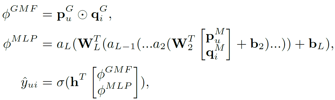
- Using the same embedding layer for both architectures and combining the output (Equation 10) - The issue with this architecture is the limitation of the performance of the fused model. GMF and MLP must use the same size of embeddings; for datasets where the optimal embedding size of the two models varies a lot, hence limiting the performance of the model.
- Using separate embedding layer for both architectures and combining the output (Equation 11) - The embedding layer for user and item vectors is fed to the MLP model and GMF model separately. The outputs received from both models is concatenated at the last hidden layer. The complete model is termed as Neural Matrix Factorization, abbreviated as "NeuMF" shown in Figure 4.
The objective function is non-convex in nature which leads to the gradient descent optimization to find locally-optimal solutions. To circumvent this, both the models - GMF and MLP are initialized by pretrained weights to converge faster and efficiently. The only change happens in the concatenation stage in which we introduce a hyperparameter α which determines the trade-of between the two pre-trained models. The optimizer used for a pretrained NeuMF is Adam optimizer instead of vanilla SGD as it improves convergence and eases hyperparamter tuning.
Results and Discussion
Test Datasets Description
The proposed NeuMF architecture is tested on two publically accessible datasets, MovieLens and Pinterest. The Movielens dataset is an explicit feedback dataset based on ratings is transformed into implicit dataset by marking the entires with a rating as 1 and 0 otherwise. Pinterest dataset is very large and sparse hence a subset of the dataset with more than 20 interactions(pins) is filtered and used.
Evaluation Metrics
For evaluating item recommendation Leave One Out Cross Validation (LOOCV) is used. Hence, the latest interaction of each user is used as testing set, leaving the remaining interactions for all users as training set.
For evaluating the ranked list of recommended items, Hit Ratio (HR) and Normalized Discounted Cumulative Gain (NDCG) are used. The HR intuitively measures whether the test item is present on the top-10 list, and the NDCG accounts for the position of the hit by assigning higher scores to hits at top ranks. The final score for each user is an average of both.
Parameter Setting
The following hyperparamters were set during the testing phase after cross-validation using randomly sampling one interaction of each user -
- All NCF models are learnt by optimizing the log loss which where we sampled 4 γ- instances per γ instance.
- For NCF models that are trained from scratch, we randomly initialized model parameters with a Gaussian distribution with a mean of 0 and standard deviation of 0.01.
- Optimizing the model was performed with mini-batch Adam optimizer
- Tests were conducted on the batch size of [128, 256, 512, 1024] with the learning rates of [0.0001 ,0.0005, 0.001, 0.005].
- The last hidden layer of NCF determines the model capability, so, we term it as predictive factors and evaluated the factors of [8, 16, 32, 64]. It is worth noting that large factors may cause overfitting and degrade the performance.
- For the NeuMF with pre-training, α was set to 0.5 which depicts equal contribution of GMF and MLP to the final prediction.
Performance Comparison with Baselines
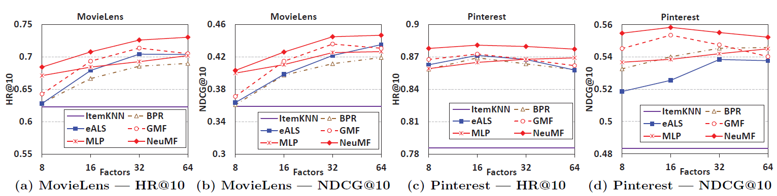
4 baseline algorithms were compared with GMF, MLP and the fused NeuMF model. The baselines were ItemPop, ItemKNN, BPR and eALS. The comparison of their performances of the test dataset is shown in Figure 5. The worst performer was ItemPop and was omitted from the visualizations. NueMF outsmarts the state-of-the-art algorithms eALS and BPR by a large margin. For Pinterest dataset, at a predictive factor of 8 itself performs way better than eALS and BPR at a factor of 64. Additionally, the results of NeuMF crosses both GMF as well as MLP. Hence, proving that fusing linear and non-linear model suffiently captures the user-item interactions in the best way. MLP slightly underperforms as compared to GMF but that can be due to lesser hidden layers and a deeper network would give better results.
Coming to the comparison of the baselines when looking at top K ranked recommendations (Figure 6), NeuMF outsmarts all other baselines for values of K while getting a tough competition from eALS and BPR. Similar to Figure 5, ItemPop performs the worst proving that recommending popular items doesn't give good results but personalized recommendations work better.
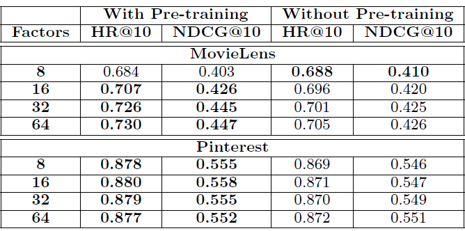
Pretraining Improvement
The Figure 7 records the results of the testing the model on pretrained and non-pretrained NeuMF. For the lowest predictive factor of 8, non-pretrained model gives better scores but that is very slightly higher than its counterpart. The table clearly proves the advantage of pretraining the fused model for 4 predictive factors.
Log Loss with Negative Sampling
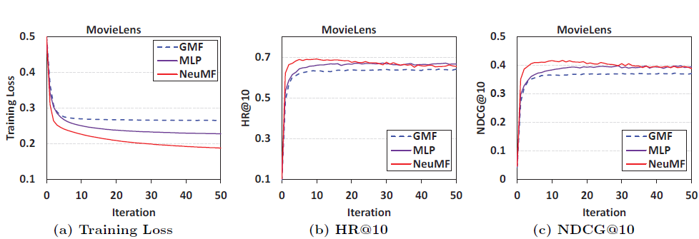
As explained above, log loss is used as the loss function in NeuMF and the problem is transformed into a binary classification problem. The training loss and performance improvement trends w.r.t increasing interactions is represented in Figure 8. It depicts that, with increasing interactions training loss decreases, hence making a better recommender system. The highest jumps in lowering the training loss happened in the initial 10 iterations which then became a plateau. Second, among the three NCF methods, NeuMF achieves the lowest training loss, followed by MLP, and then GMF. The recommendation performance also shows the same trend. This proves the rationality, correctness and effectiveness of loss loss for learning though implicit data.
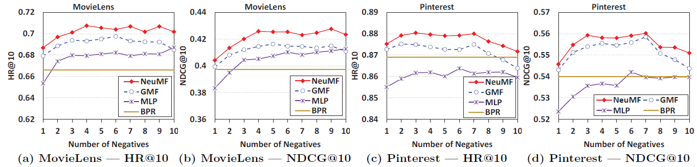
To understand the effect of different sampling ratios(the number of negative samples per positive sample) on NCF methods, the plots shown in Figure 9 are created. It shows that sampling 1 positive sample for a negative sample gives the least score and is hence least efficient. For both datasets, the optimal sampling ratio is around 3 to 6. On Pinterest, we find that when the sampling ratio is larger than 7, the performance of NCF methods starts to drop. It reveals that choosing the sampling ratio too aggressively may adversely hurt the performance.
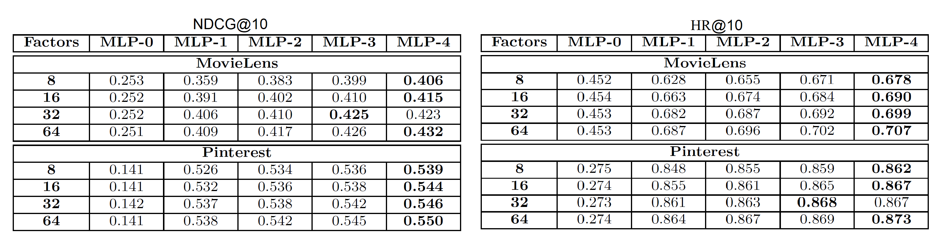
Does deep learning give better recommendations?
Since there is very less work done on usage of deep learning methods in collaborative filtering, this is an important question to address. Towards this, an experiment of changing the number of MLP layers in the MLP model of NeuMF is performed with no of MLP layers randing from 0(linear model) to 4. Here, the number of layers are counted excluding the embedding layer. Figure 10 records these results. It is noteworthy that for all predictive factors increasing the no. of layers resulted in improved performance except for factor of 32 on Pinterest dataset. The difference is very little and hence can be ignored. These results indicate a very positive response towards usage of deep learning for collaborative filtering of implicit feedback. To verify the cause of improvement can be attributed to non-linearity, the authors have noted results by stacking linear layers on top of other by using identity activation function and the performance was observed to be lower. Hence, verifying that non-linearity brought by deep neural networks is the cause of improved performance. Another key observation is that MLP-0(linear model) has lowest scores for all factors proving that a simple concatenation of user and item latent vectors is not sufficient to understand their interaction.
Conclusion
This research marks the beginning of using deep neural networks for collaborative filtering using implicit data. We started by proving the inability of linear models and simple inner product operation to understand the complex user-item interactions. We have then talked about the NCF architecture in its 3 instantiations - GMF, MLP and NeuMF. Later, we have proved that NCF is the generalization of MF. Various experiments on the NCF architecture have proved its state-of-the-art capabilities on 2 test datasets - Pinterest and MovieLens.
Outro
This marks the end of our paper explanation of Neural Collaborative Filtering. It opens up great avenues of deep learning research in this space.
Coming up next is the implementation of NCF using Pytorch