Reinforcement learning (RL) is a field of machine learning that is concerned with learning how to make decisions by observing the environment and receiving feedback in the form of rewards or penalties. Policy gradient is a popular approach in RL that is used to learn a policy function that maps states to actions, by directly optimizing the expected return of the policy.

In this article, we will discuss the basics of policy gradient, including the motivation behind it, the mathematical formulation, and some of the popular algorithms used in practice.

Motivation

The goal of RL is to learn a policy function that maximizes the expected cumulative reward obtained over a sequence of actions. However, the optimal policy may not be easy to compute directly, especially when the state and action spaces are large or continuous. In such cases, it may be more feasible to learn the policy by following a gradient-based optimization approach.

The policy gradient approach uses the gradient of the expected cumulative reward with respect to the policy parameters to update the policy. This allows us to learn a policy function that directly maximizes the expected return, without explicitly computing the optimal policy.

Mathematical Formulation

Policy

Let's define the policy as π_θ(a | s), where θ is the set of policy parameters.

Objective

The objective of policy gradient is to maximize the expected cumulative reward J(θ) with respect to θ.

J(θ) = E_{τ ∼ πθ} [R(τ)]

J(θ): the expected cumulative reward
τ: a trajectory of states and actions generated by following the policy π_θ
R(τ): the total reward obtained by following that trajectory
E_{τ ∼ πθ}: the expectation taken over all possible trajectories generated by following the policy π_θ

Gradient

The policy gradient algorithm updates the policy parameters θ in the direction that maximizes J(θ), using the gradient of J(θ) with respect to θ. The gradient of J(θ) is given by:

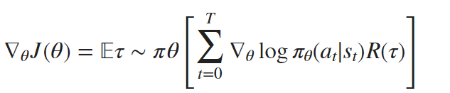
∇_θ J(θ): the gradient of the expected cumulative reward with respect to θ
∇_θ log π_θ(a_t | s_t): the gradient of the logarithm of the policy π_θ with respect to θ
T: the time horizon of the trajectory τ
R(τ): the total reward obtained by following the trajectory τ
(s_t, a_t): the state-action pairs at time stamp t
E_{τ ∼ πθ}: the expectation taken over all possible trajectories generated by following the policy π_θ

Estimating the Gradient

We can estimate the gradient of J(θ) using Monte Carlo simulation. Specifically, we can generate a set of trajectories τ_i by following the policy π_θ, and estimate the gradient using the sample average:

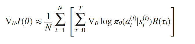
N: the number of trajectories used in the estimate
(s_t⁽ⁱ⁾, a_t⁽ⁱ⁾): the state-action pairs in trajectory τ_i

Gradient Update Rule

The gradient update rule for policy gradient is:

θ ← θ + α ∇_θ J(θ)

θ: the policy parameters
α: the learning rate
∇_θ J(θ): the gradient of the expected cumulative reward with respect to θ

The update rule moves the policy parameters θ in the direction that increases the expected cumulative reward J(θ), at a step size controlled by the learning rate α.

Advantages of Policy Gradient

Policy gradient has several advantages over other reinforcement learning algorithms:

1. Policy gradient can directly optimize policies in continuous action spaces, whereas other methods like Q-learning are limited to discrete actions.
2. Policy gradient can learn stochastic policies, which can be useful for exploration.
3. Policy gradient can handle non-stationary environments, where the optimal policy changes over time.

Disadvantages of Policy Gradient

However, policy gradient also has some disadvantages:

1. Policy gradient can be sample inefficient, since it requires a large number of samples to estimate the gradient accurately.
2. Policy gradient can suffer from high variance, since the gradients are estimated using Monte Carlo simulation.
3. Policy gradient can get stuck in local optima, especially if the policy is highly stochastic.

Extensions of Policy Gradient

There are several extensions of policy gradient that aim to address its limitations:

• Actor-Critic: Actor-critic methods combine policy gradient with value function approximation, which can reduce the variance of the gradient estimates and speed up learning.
• Trust Region Policy Optimization (TRPO): TRPO constrains the step size of the policy update to ensure that the new policy is close to the old policy, which can improve stability and reduce the risk of performance degradation.
• Proximal Policy Optimization (PPO): PPO modifies the objective function of policy gradient to discourage large policy updates, which can also improve stability and reduce the risk of performance degradation.

In summary, policy gradient is a powerful reinforcement learning algorithm that can directly optimize policies in continuous action spaces and learn stochastic policies. However, it can be sample inefficient, suffer from high variance, and get stuck in local optima. Extensions like actor-critic, TRPO, and PPO aim to address these limitations and improve the performance of policy gradient in practice.

Conclusion

Policy gradient is a powerful approach in RL that allows us to learn a policy function that directly maximizes the expected return. The policy gradient approach uses the gradient of the expected cumulative reward with respect to the policy parameters to update the policy. There are several algorithms used in practice to optimize the policy using policy gradient, including Actor-Critic, TRPO and PPO. Each algorithm has its own advantages and disadvantages, and the choice of algorithm depends on the specific task and requirements.