When we reward our kids, or pets for perfectly carrying out an assigned task, or when we scold them for not doing what was expected of them, we are actually engaging them in a reinforcement kind of leaning; each time they are rewarded (positive reward), we are reinforcing the very action they performed, and when they are scolded (negative reward), we are discouraging that very action.

Here is an excerpt from the proposal summited to the Rockefeller foundation in 1956 by a group of ten scientist who convened at Dartmouth College:** We propose a 2 month, 10 man study of artificial intelligence be carried out…..The study is to proceed on the basics of the conjecture that every aspect of learning or any other feature of intelligence can in principle be so precisely described that a machine can be made to simulate it**. What this actually means is that we can model the rewarding behaviour exhibited by man in machines (read robot, or some other software programs), and use them to perform task originally reserved for human beings.

In this article, we will be covering the Q-function, which is a value based learning algorithm in reinforcement learning.

In reinforcement learning,

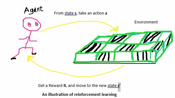
The Agent is our machine (read robot), who explores and exploits the external environment by taking actions, moving to a new state, and getting rewards.

The Environment is any external location where the agent tries to learn on its own how it can navigate across it and carry out a stipulated task.

The State is the very location in which our robot is at a particular point in time.

The Action is what the robot did to move to the new location or state in the environment

The Reward is the prize value for taking an action.

Q-FUNCTION

The Q –function makes use of the Bellman’s equation, it takes two inputs, namely the state (s), and the action (a). It is an off-policy / model free learning algorithm. Off-policy, because the Q- function learns from actions that are outside the current policy, like taking random actions. It is also worth mentioning that the Q-learning algorithm belongs to a temporal differential learning-TD. The Temporal Difference plays its part by helping the agent to calculate the Q-values with respect to the changes in the environment over time.

In Q-learning, as the agent learns and gathers insight in the environment, it stores it in a table as a reference guide for future actions, this table is called Q-table. The values stored represents the long-term reward values for specific actions taking in a specific state. Now, based on the value in a specific grid in the Q table, the Q learning algorithm will guide the Q agent to which action to choose in a particular situation to get the best expected reward.
Generally, before updating with new q-values, the q-table or matrix is first initialized to zeros.

We use code as this

Import numpy as np
Q = np.zeros(state, action)

This numpy codes sets the entire reward table or matrix to zeros.

The Q in Q-learning represent quality, the algorithm seeks to know how useful a particular action is to be able to rake in maximum future reward, this implies that the Q-function is interested in quality of the action that is necessary to move to a new state, rather than calculating the value of the state.

Let us now create a scenario where our agent will need to get to the location with an item in the table below, starting from point A; it will be difficult for the agent to perform this task, because the agent doesn’t know what path to take, hence we need to guide it with some form of footprint it will follow.

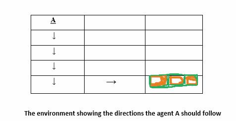
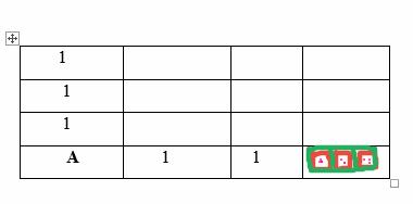
Table with footprint for the agent

Now, let us assume we put the values 1 as the guide and footprint for the agent, there comes a time in the grid/environment when the agent will run into decision issues, as in the case above, here we have the same values on the left and right side. How is this agent going to decide which path is optimal relative to the end location? This is where the Bellman’s equation takes over for a smooth operation and guidance.

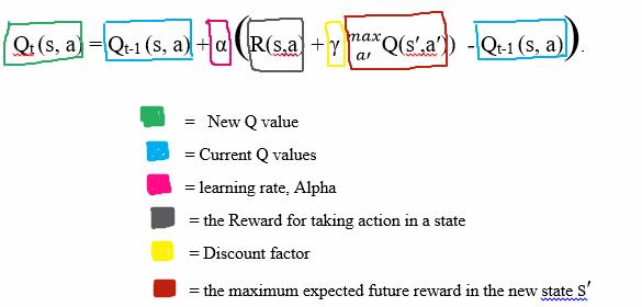
Bellman’s equation:

$$V(s){=}_a^{\max }(R(s,a)+\gamma (V(s\text{'}))$$

• s = The very state in time
• a = the action taking to move to the next state
• s′ = the state we achieved moving the agent from s
• 𝜸 = discount factor
• R(s, a) = the reward function that takes a state s and action a and returns a
  reward value
• V(s) = this is the value of being in a particular state in time.

Here we have a grid marked with unknown value - blue asterisk, assuming we take the discount factor = 0.85, its value at the start location using Bellman’s equation will be-

$$V(s){=}_a^{\max }(0+0.85*1)=0.85$$

Note: Although the agent in this case can see that a reward “1” is next to the end_location with the highest reward, but it cannot go to that grid (read state) the grid is not directly accessible for now, hence, in that instance, R(s,a) = 0; On the others hand, this agent knows the value of this very future state , that is V(s′) = 1. Consequently, with this information at hand, we can calculate the various states from the start location to the end location.
We will get these state values: 0.522, 0.6141, 0.7225, and 0.85, as tabulated below:

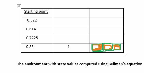
If we compute all the state values in the table, the agent can now easily go to the end location using these values as a guide. In the light of these, it is now obvious that the equation basically gives us the value of any state in time.
With that said, it is worth remembering that in reality, our environment is filled with a lot of uncertainties, and some level of randomness, this makes it difficult for things to function exactly as expected. With probability now as a factor, we move into Markov Decision Process MDP.

Markov Decision Process is a discrete time stochastic control process, it provides a mathematical framework for modelling decision making in situations where outcomes are partly random and partly under the control of a decision maker

Using our Bellman’s equation as usual:

$$V(s){=}_a^{\max }(R(s,a)+\gamma (V(s\text{'}))$$

Taking into account the probabilities of moving from the current state s, taking an action a to get into the future state s′ = P(s, a, s′), our Bellman’s equation becomes:

$$V(s){=}_a^{\max }(R(s,a)+\gamma {\displaystyle \sum _{s\text{'}}P(s,a,s\text{'})}(V(s\text{'}))$$

Where:

$${\displaystyle \sum _{s\text{'}}P(s,a,s\text{'})}=$$

• the expected circumstance in which the agent gets into uncertainties or randomness.

Recall from our definition of Q learning function - that the Q-function is interested in quality of the action that is necessary to move to a new state, rather than the value of the state, also, that it belongs to a temporal differential learning TD, and bringing to mind that, in the original Bellman’s equation, we were taking all maximum values resulting from taking certain good actions; this can be understood to mean that V(s) is the maximum of all the possible values of Q(s, a); therefore, if we imagine this in terms of quality of an action, with regard to the q-function, we can replace V(s) with Q(s,a) in the equation:

$$Q(s,a)=R(s,a)+\gamma {\displaystyle \sum _{s\text{'}}P(s,a,s\text{'})}(V(s\text{'}))$$

Substituting further, we get:

$$Q(s,a)=R(s,a)+\gamma {{\displaystyle \sum _{s\text{'}}P(s,a,s\text{'})}}_{a\text{'}}^{\max }Q(s\text{'},a\text{'}))$$

Furthermore, we will bring component of the temporal difference into play, because we are not very sure of the exact reward we will get in the future state s′; to do this, we will subtract the known q-value from the new q-value –

$$TD(a,s)=R(s,a)+\gamma {{\displaystyle \sum _{s\text{'}}P(s,a,s\text{'})}}_{a\text{'}}^{\max }Q(s\text{'},a\text{'}))-Q(s,a)$$

                           **↑ This is the New Q(s,a)*

Once we get the New Q(s,a), an update in done on the q-table using this equation:

$$Q_t(s,a)=Q_{t-1}(s,a)+\alpha T{D}_t(a,s)$$

Where:

α = stands for the learning rate, this regulates how fast an agent adapts to the uncertainties or random changes encountered in the environment.

$$Q_t(s,a)=The\_Current\_q\_value$$ $$Q_{t-1}(s,a)=The\_previous\_q\_value$$

Finally, substituting for TD in the updated equation, we get:

$$Q_t(s,a)=Q_{t-1}(s,a)+\alpha \left(R(s,a)+{\gamma }_{a\text{'}}^{\max }Q(s\text{'},a\text{'})-Q_{t-1}(s,a)\right)$$

Now, let us go over and try our hands on some Python implementation of Q-learning

Task for the Agent:

In this task, there are 12 different apartment in a building, each apartment has a key to a treasure, but one of the apartment got the golden key to the treasure. The location of the golden key changes at random. We are to build a robot to get the apartment with the golden key using the shortest route possible, starting from any given location it chooses on its own.

Here is the building with the 12 apartment:

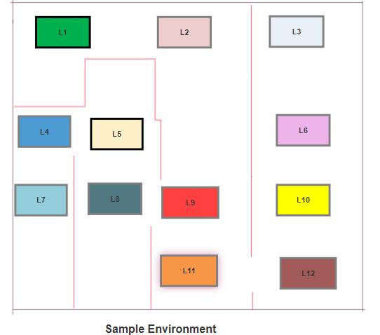
From the picture, there are obstacles between locations, hence the robot will have to navigate through these obstacles en-route the apartment of interest.

Note: The Agent in this scenario is the robot, the Environment is the building, and the apartment (read location) is the State. What We mean is that,the location a robot stands at a particular point in time, is the state.

The Actions: From the scenario, each action taken by the robot will move it to the next apartment or location, no doubt; but there are obstacles between these locations, hence for there to be a viable action, the robot should have a direct movement from one apartment to the other.

Consider this scene- the Agent is at L9, L3, and L4 at various times.

• Scene 1: The actions or direct location it can move to while at L9 = L2, L11, L8.
• Scene 2: while at L3 = L6.
• Scene 3: while at L4 = L5, L7.

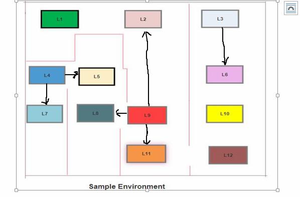
As we can see from this illustration, the sets of actions connotes sets possible state of the agent; this implies that there will be different sets of actions at different locations of the agent.

We move to the Rewards. We recall that rewards are functions of state and actions; then going by this, we now have our rewards from these sets:

• From sets of states S = 0,1,2,3,4,5,6,7,8,9,10,11
• From sets of actions A = 0,1,2,3,4,5,6,7,8,9,10,11

This implies that once the agent moves from its location directly to another location it will receive a reward. For instance, if the agent goes from L9 to L11, it receives a reward 1, but when it cannot directly get to a location, either due to the obstacles, or like in a scenario between L10 and L3 where L3 is not directly reachable from L10, then in such case, the agent will not receive a reward( zero (0) reward). This numbers (read reward) helps the agent to navigate through the entire building by sensing which location is directly reachable and which ones are not- that is 0 = not directly reachable, and 1 = reachable.

Now let us construct a reward table using this 0’s and 1’s idea.

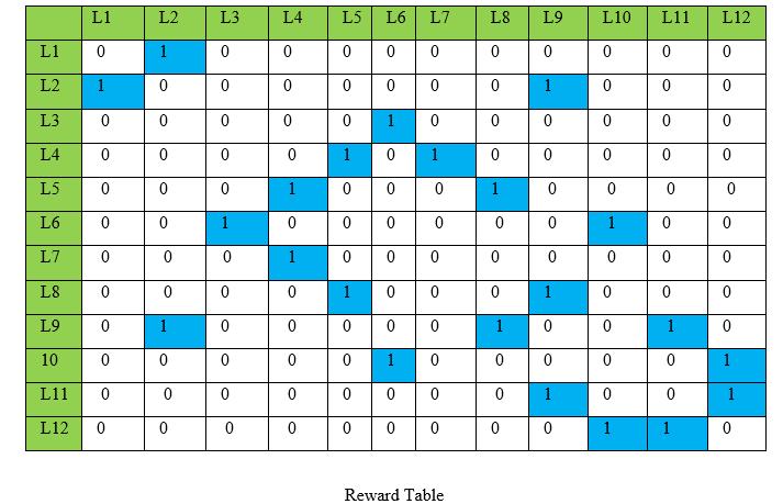
This table shows a reward matrix of all rewards the agent can possibly get from going from one state to another.

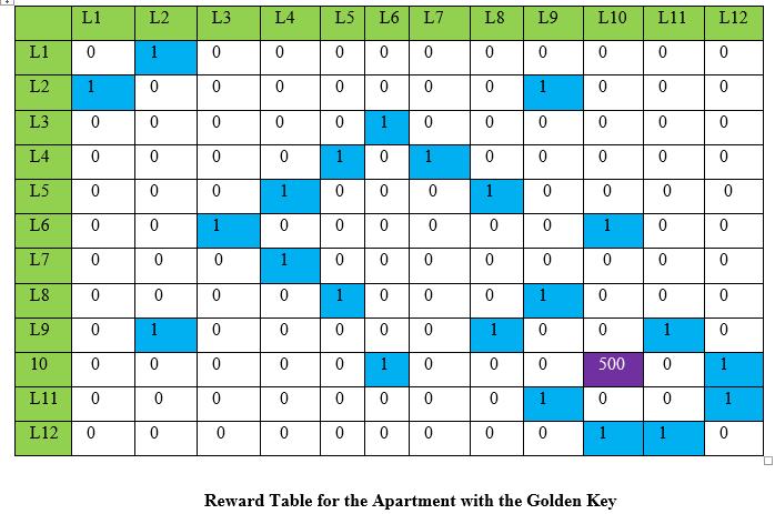
Recall that we were to assign of one the apartment with the golden key, now in other to make this possible, we will differentiate the reward at this location in other for the agent to be able to identify the apartment (read location). Here we assign a reward of 500 at location L10, L10:

What we have succeeded in all the pictorial illustrations above, was to bring to perspective the key components we will be utilizing in our Python implementation of Q-learning.

Now lets hit the code

import numpy as our dependency

import numpy as np

intializing our parameters

gamma = 0.85 #discount factor
alpha = 0.9  # learning rate

# define the states(Map each of the locations to numbers(states))
    location_to_state = {'L1' : 0,
    'L2' : 1,
    'L3' : 2,
    'L4' : 3,
    'L5' : 4,
    'L6' : 5,
    'L7' : 6,
    'L8' : 7,
    'L9' : 8,
    'L10': 9,
    'L11': 10,
    'L12': 11
    }
# define our action(actions here represents the transition to the next state:)
    actions = [0,1,2,3,4,5,6,7,8,9,10,11]
    #define the reward (get the reward table)
    rewards = np.array(
              [[0,1,0,0,0,0,0,0,0,0,0,0],
              [1,0,0,0,0,0,0,0,1,0,0,0],
              [0,0,0,0,0,1,0,0,0,0,0,0],
              [0,0,0,0,1,0,1,0,0,0,0,0],
              [0,0,0,1,0,0,0,1,0,0,0,0],
              [0,0,1,0,0,0,0,0,0,1,0,0],
              [0,0,0,1,0,0,0,0,0,0,0,0],
              [0,0,0,0,1,0,0,0,1,0,0,0],
              [0,1,0,0,0,0,0,1,0,0,1,0],
              [0,0,0,0,0,1,0,0,0,0,0,1],
              [0,0,0,0,0,0,0,0,1,0,0,1],
              [0,0,0,0,0,0,0,0,0,1,1,0]])

# Now,lets inverse mapping from the states back to original location indicators.
    #since it will help identify locations using their current state
    state_to_location = dict((state,location) for location,state in   
    location_to_state.items())

    print(state_to_location)

define our function : get_optimal_route(it takes two argument:starting_location end_location in the building. It will return the optimal location in the form of an ordered list with letters to represent each location.

    def get_optimal_route(starting_location,end_location):

    # lets make a copy of the reward matrix, we dont want to alter the origianl  
    #table.
     
        rewards_copy = np.copy(rewards )
        print("rewards_copy is :","\n", rewards_copy)
        print()

        # create a random location for the golden key
        golden_key_location = np.random.randint(0,11)
        list_location_to_state = list(location_to_state.keys())
        end_location = list_location_to_state[golden_key_location]
        print(end_location)

        # Get the ending state corresponding to the ending location as given
 
        ending_state = location_to_state[end_location]
        print(ending_state)
        print()
    
        # Automatically set the priority of the
        # given ending state to the highest one
        rewards_copy[ending_state,ending_state]= 500
        print(rewards_copy)

        # Initialize Q -Values to zero
        Q = np.array(np.zeros([12,12]))
    
        # We will explore the environment for a while, by looping it through 1000   
        #times.
        #We will then pick a state randomly from the set of states we defined above,
        # lets call "current_state".
        for i in range(1000):
            # Pick up a state randomly
            current_state = np.random.randint(0,12)
        
            # iterating through the rewards matrix,we get the states that are  
            #directly reachable
            # from the randomly chosen current state and we will then assign those 
            #states in a list
            # called "playable_actions".
            playable_actions = []    
            for j in range (12):
                if rewards_copy[current_state,j]>0:
                    playable_actions.append(j)
                
                    # Pick an action randomly from the list of playable actions 
                    #leading us to the next state
                    next_state = np.random.choice(playable_actions)
                    # Compute the temporal difference
                    # Note: The "action" here exactly refers to going to the "next 
                    #state"
                    TD = rewards_copy[current_state,next_state ] + 
           gamma*Q[next_state ,np.argmax(Q[next_state])] Q[current_state,next_state]
                    # Update the Q-Value using the Bellman equation
                    Q[current_state,next_state]+= alpha*TD
        # Initialize the optimal route with the starting location
        route = [starting_location]
        # we at this juncture will have to set the next_location to the 
        #starting_location, reason being that
        # we dont know what move the agent will be making at this moment
        next_location = starting_location

        # A "while loop will be goog for iteration in this case",
        # we don't know the exact number of iterations required to reach to the 
        #final location.
        while(next_location != end_location):
            # pickup the starting state
            starting_state = location_to_state[starting_location]
            # pickup the highest Q-value pertaining to starting state
            next_state = np.argmax(Q[starting_state])
            # get the letters of the locations corresponding to the next state
            next_location = state_to_location[next_state]
            route.append(next_location)
            # Now we update the starting location for the next iteration
            starting_location = next_location

        return route

    print(get_optimal_route("L12","L1"))

We have finally come to end of this article, I do hope it gave you some new insight, and perspective regarding reinforcement learning, and Q-learning function in particular.

My appreciation to Aditya Chatterjee of OpenGenus whose guidance has been very helpful to my reinforcement learning journey, and Sayak Paul whose article on Q-learning gave me a nice perspective in this area.