Open-Source Internship opportunity by OpenGenus for programmers. Apply now.
Reading time: 50 minutes
Stacked generalization (or simply, stacking or blending) is one of most popular techniques used by data scientists and kagglers to improve the accuracy of their final models. This article will help you get started with stacking and achieve amazing results in your journey of machine learning. After reading this article you will knowledge about the following concepts:
- Baseline prediction algorithms
- Concept of stacking
- Why and when to use stacking ?
- How to select submodels for stacking?
- Why correlation between submodels to be low?
- Stacked dataset description
- Code for stacking
Baseline prediction algorithms
When given a new dataset, it is often useful to apply a baseline prediction algorithm (BPA) whose accuracy can be used as a point of comparison for more advanced algorithms that will be trained on the dataset. Two of the most common BPA use are random prediction algorithm and zero rule prediction algorithm. Let’s see each one of them one by one.
Random Prediction Algorithm
It is perhaps the simplest algorithm to implement. Here:
- Step 1 : Store all the unique output values of the training dataset in a list.
- Step 2 : For every row in the test dataset, pick up a value from this list randomly. This random output value becomes the prediction of the random pred algo for the corresponding row of the test dataset.
That’s it! Not even any sort of training required here!
Zero Rule Prediction Algorithm
This algorithm is better than random prediction algo as it uses more information from the dataset. It makes use of a rule which depends on the type of problem, we are dealing with.
For classification problems:
Step 1 : Find the most common class in the training dataset. If there are 100 training examples of class 1 and 80 examples of class 2, then class 1 becomes the most common class.
Step 2 : For every row in the test dataset, output class 1 (most common class) as the predicted class.
For regression problems:
Step 1 : Find the a central tendancy (mean or median) of the output values of the training dataset.
Step 2 : For every row in the test dataset, output the central tendancy as predicted output value.
We will be using zero rule prediction algorithm to get baseline accuracy on our dataset.
Concept of Stacking
Stacked generalization was introduced by Wolpert in a 1992 paper. The basic idea behind stacking is to combine the predictions of 2 or more models to get predictions of higher accuracy than the previous submodels. Here’s a diagram to give you a better idea :
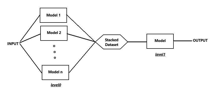
As you can see in the dig., the models in the first layer (model1 , model2 etc) are the submodels whose predictions are combined to form a new dataset (called stacked dataset). This stacked dataset is given as input to the aggregator model which makes final predictions. The dig shows only two layers of models stacked one above the other. But we can also add more layers of models to get even better results. Although we have to keep in mind the computational power we have in our computers (more on that later). Let’s see how 3 layers stacked together would look like :
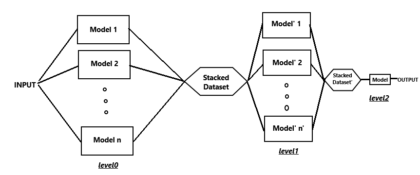
Why does stacking give such great results and when to use it?
In order to explain why stacking gives such great results, let us go back to high school where we studied the chapter Probability. Suppose, we trained 3 models on our dataset and each of them gave 70 percent accuracy on the test dataset. Now for any given row from the test dataset, following 4 cases are possible :
a) All 3 models give correct prediction
b) 2 out of three models give correct prediction
c) 1 out of 3 model give correct prediction
d) None of them give correct prediction
Let us see the probability of each case:
P(a) = 0.7 * 0.7 * 0.7 = 0.343
P(b) = (0.7 * 0.7 * 0.3) * 3 = 0.147 * 3 = 0.441
P(c) = (0.7 * 0.3 * 0.3) * 3 = 0.063 * 3 = 0.189
P(d) = 0.3 * 0.3 * 0.3 = 0.027
Now, in case a and b , the majority of the models predict correctly so the ensembler in these to cases will give the correct prediction. The probability of these 2 cases, combined, is 0.784. In the other 2 cases, the majority of models, predict incorrectly whose probability is 0.189 + 0.027 = 0.216. Thus, we see that the ensembler gives the correct outout 78.4 percent of the time which is way more than 70 percent accuracy of submodels.
Now that we have seen why stacking gives such great results, let us see when to use it. Stacking takes up quite a bit of computational power and time. So we should use it only when we have access to computers with high computational powers and also when we have enough time.
How to select submodels for stacking?
The submodels that we choose need not be the best possible models for the given model. We should also focus on choosing models that are weakly correlated to each other. We can do so by choosing algorithms that very different internal representations (trees compared with instances) or are trained on different representations or projections of the data.
Why should the correlation be low between submodels?
This can be explained with a very simple example. Let the correct output be all one’s.
Suppose we have 3 models, whose accuracy is :
1111111100 = 80% accuracy
1111111100 = 80% accuracy
1011111100 = 70% accuracy.
Now, if we ensemble these models, the resulting output is with majority vote :
1111111100 = 80% accuracy.
Now let us take the following 3 models:
1111111100 = 80% accuracy
0111011101 = 70% accuracy
1000101111 = 60% accuracy
After ensembling these models with majority voting, the result is:
1111111101 = 90% accuracy.
Thus we see, less correlated models produce better results.
It is usually desirable that the level 0 generalizers are of all “types”, and not just simple variations of one another (e.g., we want surface-fitters, Turing-machine builders, statistical extrapolators, etc., etc.). In this way all possible ways of examining the learning set and trying to extrapolate from it are being exploited. This is part of what is meant by saying that the level 0 generalizers should “span the space”.
"[…] stacked generalization is a means of non-linearly combining generalizers to make a new generalizer, to try to optimally integrate what each of the original generalizers has to say about the learning set. The more each generalizer has to say (which isn’t duplicated in what the other generalizer’s have to say), the better the resultant stacked generalization." - Wolpert (1992) Stacked Generalization
Stacked dataset description
Now let us see how the stacked dataset, the one we train our aggregator model on, looks like. The predictions of each model are taken as one column of the stacked dataset. Once we have the predictions of each submodel “stacked” column by column, we add the last column which contains the actual output predictions. Thus every row in this dataset represents output of each model corresponding to a row in the training dataset and the last cell of each row in the stacked dataset contains the actual output.
Code
We will be working on the famous titanic survival dataset. The description of the dataset and my complete code can be found here.
Let's first import the libraries required.
# Load in our libraries
import pandas as pd
import numpy as np
import re
import sklearn
import xgboost as xgb
import seaborn as sns
import matplotlib.pyplot as plt
from sklearn.model_selection import StratifiedKFold
%matplotlib inline

from sklearn.metrics import accuracy_score
from sklearn.model_selection import GridSearchCV
from sklearn.metrics import precision_score
from sklearn.metrics import recall_score

import plotly.offline as py
py.init_notebook_mode(connected=True)
import plotly.graph_objs as go
import plotly.tools as tls

import warnings
warnings.filterwarnings('ignore')

# Going to use these 5 base models for the stacking
from sklearn.ensemble import (RandomForestClassifier, AdaBoostClassifier,
                              GradientBoostingClassifier, ExtraTreesClassifier)
from sklearn.linear_model import LogisticRegression
from sklearn.svm import SVC
from sklearn.model_selection import KFold
import os
print(os.listdir("../input"))
Next step is dataset exploration. A part of it is already done. So not much to be done here.
print ("\ntotal number of datapoints : 891")
print ("\ncabin number has many missing values")

#reading training dataset

feature_list=['PassengerId','Pclass','Name','Sex', 'Age','SibSp','Parch','Ticket','Fare','Cabin','Embarked']

df_train_features=pd.read_csv("../input/train.csv",usecols=feature_list)
df_train_labels=pd.read_csv("../input/train.csv",usecols=['Survived'])

df_test_features=pd.read_csv("../input/test.csv",usecols=feature_list)

df_train_features.head()
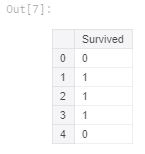
df_train_labels.head()
df_test_features.head()
Next step is data pre-processing.
#DATA PRE-PROCESSING

#replacing 'male' with 1 and 'female' with 0 in the 'sex' column
df_train_features=df_train_features.replace('male',1)
df_train_features=df_train_features.replace('female',0)

df_test_features=df_test_features.replace('male',1)
df_test_features=df_test_features.replace('female',0)

#extracting the numerical part of the ticket number
#c=5
for s in df_train_features.iloc[:,7]:
    if isinstance(s,str):
        value=[int(s) for s in s.split(' ') if s.isdigit()]
        if (len(value)!=0):
            tktnum=value[0]
        else:
            tktnum=-1
        #if (c>0):
          #  c-=1
        df_train_features=df_train_features.replace(s,tktnum)
        #df_test_features=df_test_features.replace(s,tktnum)

#c=5
for s in df_test_features.iloc[:,7]:
    if isinstance(s,str):
        value=[int(s) for s in s.split(' ') if s.isdigit()]
        if (len(value)!=0):
            tktnum=value[0]
        else:
            tktnum=-1
        #if (c>0):
           # c-=1
        #df_train_features=df_train_features.replace(s,tktnum)
        df_test_features=df_test_features.replace(s,tktnum)

#In 'embarked' column, replacing 'S' by 1,'C' by 2 and 'Q' by 3
df_train_features['Embarked'] = df_train_features['Embarked'].replace({"S":1.0,"C":2.0,"Q":3.0})
df_test_features['Embarked'] = df_test_features['Embarked'].replace({"S":1.0,"C":2.0,"Q":3.0})

#Extracting only the surnames
for s in df_train_features.iloc[:,2]:
    if (len(s)!=0):
        value=[s for s in s.split(',')]
        surname=value[0]
    df_train_features=df_train_features.replace(s,surname)
    df_test_features=df_test_features.replace(s,surname)
#finding the list of unique surnames present and assigning them a numerical value
ls=df_train_features.Name.unique()
df_train_features=df_train_features.replace(ls,range(len(ls)))
ls=df_test_features.Name.unique()
df_test_features=df_test_features.replace(ls,range(len(ls)))

#For cases where a passenger has more than one cabin number, extra features will be added.
#If a person has two cabins, then 4 features will be added. 2 for alpha. part and 2 for numerical part.
#splitting cabin number in two parts: cabin1 : contains the alphabetical part and cabin2 : contains the numerical part

#first let us find the maximum number of cabins a passenger has.
Max=0
for s in df_train_features.iloc[:,9]:
    if isinstance(s,str):
        value=[s for s in s.split(' ')]
        if (Max<len(value)):
            Max=len(value)
print ('maximum number of cabins a passenger has : ',Max)

#now let us add the required number of features with default values for each row. Later on the value of a row will be changed as
#'needed'
x=range(Max)
for i in x:
    df_train_features.loc[:,'ap'+str(i)]=-1
    df_train_features.loc[:,'np'+str(i)]=-1
    df_test_features.loc[:,'ap'+str(i)]=-1
    df_test_features.loc[:,'np'+str(i)]=-1
    feature_list.append('ap'+str(i))
    feature_list.append('np'+str(i))
#now let us fill in the apprpriate values in these new columns
ap=11
np=12
rowin=0

for s in df_train_features.iloc[:,9]:
    if isinstance(s,str):
        #print (s)
        #print (type(s))
        value=[s for s in s.split(' ')]
        for cn in value:
            #print (cn[0])
            #print (cn[1:])
            #print (ap)
            df_train_features.iloc[rowin,ap]=ord(cn[0])
            #df_test_features.iloc[rowin,ap]=ord(cn[0])
            if (cn[1:]!=''):
                df_train_features.iloc[rowin,np]=int(cn[1:])
                #df_test_features.iloc[rowin,np]=int(cn[1:])
            else:
                df_train_features.iloc[rowin,np]=-1
                #df_test_features.iloc[rowin,np]=-1
            ap+=2
            np+=2
    ap=11
    np=12
    rowin+=1

ap=11
np=12
rowin=0

for s in df_test_features.iloc[:,9]:
    if isinstance(s,str):
        #print (s)
        #print (type(s))
        value=[s for s in s.split(' ')]
        for cn in value:
            #print (cn[0])
            #print (cn[1:])
            #print (ap)
            #df_train_features.iloc[rowin,ap]=ord(cn[0])
            df_test_features.iloc[rowin,ap]=ord(cn[0])
            if (cn[1:]!=''):
                #df_train_features.iloc[rowin,np]=int(cn[1:])
                df_test_features.iloc[rowin,np]=int(cn[1:])
            else:
                #df_train_features.iloc[rowin,np]=-1
                df_test_features.iloc[rowin,np]=-1
            ap+=2
            np+=2
    ap=11
    np=12
    rowin+=1


#finally removing the original 'cabin' column
df_train_features=df_train_features.drop(columns=['Cabin'])
df_test_features=df_test_features.drop(columns=['Cabin'])
#removing from features list as well
del feature_list[feature_list.index('Cabin')]

#replacing all the missing values in age column by mean age
mean_age=df_train_features['Age'].mean()
df_train_features['Age']=df_train_features['Age'].fillna(mean_age)
df_test_features['Age']=df_test_features['Age'].fillna(mean_age)

#there are two nan values present in 'Embarked' column. we are replacing it with median value
median=df_train_features['Embarked'].median()
df_train_features['Embarked']=df_train_features['Embarked'].fillna(median)
df_test_features['Embarked']=df_test_features['Embarked'].fillna(median)


#checking for any NAN values left
l=[]
for i in feature_list:
    x=df_test_features[i].isnull().sum().sum()
    if x>0:
        print (x)
        l.append(i)
for i in l:
    print (i)
avg_fare=df_test_features['Fare'].mean()
df_test_features['Fare']=df_test_features['Fare'].fillna(avg_fare)
df_train_features.head()
Usually, operations on dataset is performed when they are in the form of numpy arrays. So first we convert our data from pandas dataframe to numpy arrays.
#Converting dataframe to numpy arrays for further use
X=df_train_features.values
y=df_train_labels.values
X_test=df_test_features.values

print ('X.shape = %s' % str(X.shape))
print ('y.shape = %s' % str(y.shape))
print ('X_test.shape = %s' % str(X_test.shape))
Now comes our next step where we optimize our features and find out their relative importance in making predictions. We will discard the less important ones. This will help in reducing the processing time and redundancy in our dataset.
Note : Feature scaling is a method used to normalize the range of independent variables or features of data. In data processing, it is also known as data normalization and is generally performed during the data preprocessing step.
#First, let us do feature scalling so that no feature gets more importance simply based on it's numerical value

#feature scalling
from sklearn.preprocessing import MinMaxScaler
scaler=MinMaxScaler()
X=scaler.fit_transform(X)


#scaler=MinMaxScaler()
X_test=scaler.fit_transform(X_test)

#Originaly, 'y' was a column vector. Here we convert it to row vector for our #operations
new=[]
for i in y:
    for j in i:
        new.append(j)
print (new[:5])
y=new
Let us now find the relative importance by calculating their corresponding scores.
#now let us find the importance of all features using selectkpercentile
from sklearn.feature_selection import SelectPercentile, f_classif
selector = SelectPercentile(f_classif, percentile=80)#Here we select top 80 percent #features

selector.fit(X,y)
X_new=selector.transform(X)
print ('shape of X_new ',X_new.shape)
try:
    X_points = range(X.shape[1])
except IndexError:
    X_points = 1


#using previously selected features
X_test=selector.transform(X_test)
print ('X_test.shape = %s ' % str(X_test.shape))
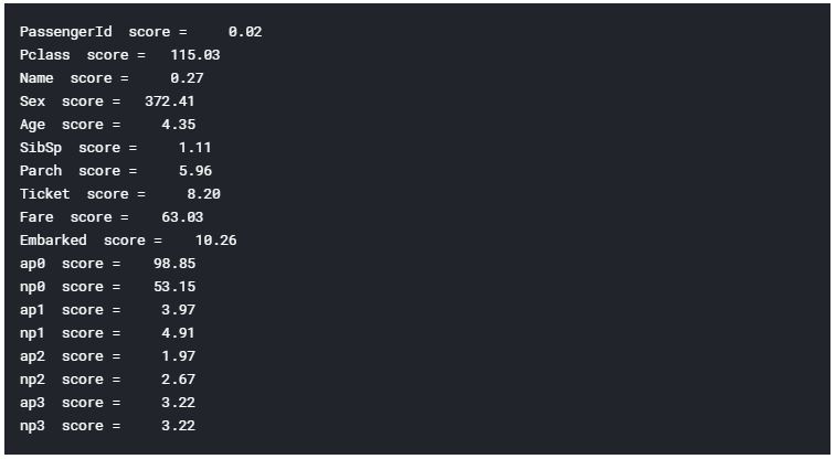
Let us have a look at the scores of the features which tell us their relative importance.
#checking out the scores of the features
score=selector.scores_.tolist()
names=list(df_train_features)
new=zip(names,score)
for i in new:
    print (i[0]," score = {:8.2f}".format(i[1]))
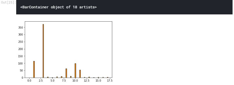
Let us plot the scores.
plt.bar(X_points , selector.scores_, width=.2,
        label=r'Univariate score ($-Log(p_{value})$)', color='darkorange',
        edgecolor='black')
Now comes the step where we apply stacking.First, we divide our data from train.csv into training and testing part (A portion of the training part will be used for cross-validating the data).
Then, let us initialize some of the commonly used variables followed by defining the level 0 classifiers.
#Splitting data into training and testing set
from sklearn.model_selection import train_test_split
features_train, features_test, labels_train, labels_test = train_test_split(X_new, y, test_size=0.30, random_state=42)

n_folds = 5
n_trees = 10

#level 0 classifiers
clfs = [
    RandomForestClassifier(n_estimators = n_trees, criterion = 'gini'),
    ExtraTreesClassifier(n_estimators = n_trees, criterion = 'gini'),
    GradientBoostingClassifier(n_estimators = n_trees),
    AdaBoostClassifier(n_estimators = int(n_trees/2))
]
Next, we write the function run() that we will perform the following tasks:
- train level 0 classifiers on our input data.
- make the stacked dataset
- train level 1 classifier to get the final output
First we call run() on our data from train.csv file only.Training, cross-validation and testing, all will be done on this data only. We take a look at the final accuracy. And then we again call run() to train our model on complete data from train.csv and produce prediction on test.csv. This time training and cross-validation is done on data from train.csv and testing is done on test.csv. We then store these predictions in a submission file which is evaluated by kaggle to give our final accuracy.
Before trying to go over this function it would be better to get an idea about the following:
StratifiedKFold : This library basically divides our data into n_folds number of parts or folds. Then we train our data on (n_folds - 1) number of folds and cross-validate it on the remaining 1 fold. Then we test this trained model to get predictions on test data. We repeat this process n_folds number of times such that we have cross-validated our model on each one of the folds atleast once. We will also have tested our model n_folds number of times. We then average all the test results to get the final result.
def run(features_train, labels_train, features_test, clfs, n_folds = 5, labels_test = None, submission = False):
    import numpy as np
    # Ready for cross validation
    skfold = StratifiedKFold(n_splits=n_folds)
    skf = list(skfold.split(features_train, labels_train))#skf is n_fold X 2 #dimensional. Each row in it contains 2 sets of indices: one telling the training #part of the data and the other telling the testing part.

    # Pre-allocate the stacked dataset
    blend_train = np.zeros((features_train.shape[0], len(clfs))) # Number of training data x Number of classifiers
    blend_test = np.zeros((features_test.shape[0], len(clfs))) # Number of testing data x Number of classifiers

    if(submission == True):
        print("\nThis run is on entire training dataset from train.csv and we will create a submission file in this run. :)")

    print ('\nfeatures_train.shape = %s' % (str(features_train.shape)))
    print ('features_test.shape = %s' % (str(features_test.shape)))
    print ('blend_train.shape = %s' % (str(blend_train.shape)))
    print ('blend_test.shape = %s' % (str(blend_test.shape)))

    # For each classifier, we train the number of fold times (=n_folds)
    for j, clf in enumerate(clfs):
        print ("\n#####################################################")
        print ('\nTraining classifier [%s]' % (str(j)))
        blend_test_j = np.zeros((features_test.shape[0], len(skf)))
        for i, (train_index, cv_index) in enumerate(skf):
            print ('Fold [%s]' % (str(i)))

            # This is the training and validation set
            #print ("train_index",train_index)
            X_train = features_train[train_index]
            Y_train = np.array(labels_train)[train_index]
            X_cv = features_train[cv_index]
            Y_cv = np.array(labels_train)[cv_index]

            clf.fit(X_train, Y_train)

            # This output will be the basis for our blended classifier to train against,
            # which is also the output of our classifiers
            blend_train[cv_index, j] = clf.predict(X_cv)
            blend_test_j[:, i] = clf.predict(features_test)

        # Take the mean of the predictions of the cross validation set
        blend_test[:, j] = blend_test_j.mean(1)
        pred = blend_test[:, j]
        #print (pred[0:5])
        #print (labels_test[0:5])
        #after averaging, the results we get would be fractions mostly which need to be converted to 1 and 0. Hence we do the following transformations
        pred[(pred >= 0.5)] = 1
        pred[(pred < 0.5)] = 0
        #print (pred[0:5])
        if (submission == False):
            #this is to test the accuracy of each level 0 0 classifier separately
            print ("accuracy_score : ",accuracy_score(labels_test,pred))
            print ('precision : ',precision_score(labels_test,pred))
            print ('recall : ',recall_score(labels_test,pred))


    print ('\nlen(labels_train) = %s' % (str(len(labels_train))))

    # Start blending!
    bclf = LogisticRegression()
    bclf.fit(blend_train, labels_train)

    # Predict now
    Y_test_predict = bclf.predict(blend_test)
    if (submission == False):
        #This is to test the accuracy of the level 1 classifier
        print ("\naccuracy_score : ",accuracy_score(labels_test,Y_test_predict))
        print ('precision : ',precision_score(labels_test,Y_test_predict))
        print ('recall : ',recall_score(labels_test,Y_test_predict))

    if (submission == True):
        x =range(892,1310)
        #creating the submission file
        submission=pd.DataFrame({'PassengerId':x,'Survived':Y_test_predict})
        print (submission.head())
        submission.to_csv(path_or_buf='submission.csv',index=False)

    print ("===========================================================================================================================")

run(features_train, labels_train, features_test, clfs, n_folds, labels_test)

# now, we train our model on complete data from train.csv file and test on data from test.csv file before we make our submission
run(X_new, y, X_test, clfs, n_folds, submission = True)
OUTPUT
features_train.shape = (623, 14)
features_test.shape = (268, 14)
blend_train.shape = (623, 4)
blend_test.shape = (268, 4)

#####################################################

Training classifier [0]
Fold [0]
Fold [1]
Fold [2]
Fold [3]
Fold [4]
accuracy_score :  0.7985074626865671
precision :  0.8275862068965517
recall :  0.6486486486486487

#####################################################

Training classifier [1]
Fold [0]
Fold [1]
Fold [2]
Fold [3]
Fold [4]
accuracy_score :  0.7798507462686567
precision :  0.776595744680851
recall :  0.6576576576576577

#####################################################

Training classifier [2]
Fold [0]
Fold [1]
Fold [2]
Fold [3]
Fold [4]
accuracy_score :  0.7947761194029851
precision :  0.9117647058823529
recall :  0.5585585585585585

#####################################################

Training classifier [3]
Fold [0]
Fold [1]
Fold [2]
Fold [3]
Fold [4]
accuracy_score :  0.8022388059701493
precision :  0.7735849056603774
recall :  0.7387387387387387

len(labels_train) = 623

accuracy_score :  0.8097014925373134
precision :  0.8488372093023255
recall :  0.6576576576576577

===========================================================================================================================
This run is on entire training dataset and we will create a submission file in this run. :)
features_train.shape = (891, 14)
features_test.shape = (418, 14)
blend_train.shape = (891, 4)
blend_test.shape = (418, 4)

#####################################################

Training classifier [0]
Fold [0]
Fold [1]
Fold [2]
Fold [3]
Fold [4]

#####################################################

Training classifier [1]
Fold [0]
Fold [1]
Fold [2]
Fold [3]
Fold [4]

#####################################################

Training classifier [2]
Fold [0]
Fold [1]
Fold [2]
Fold [3]
Fold [4]

#####################################################

Training classifier [3]
Fold [0]
Fold [1]
Fold [2]
Fold [3]
Fold [4]

len(labels_train) = 891
   PassengerId  Survived
0          892         0
1          893         0
2          894         0
3          895         0
4          896         1

===========================================================================================================================
The final accuracy that we get on kaggle is around 77 percent which is fairly accurate. You can include other models in level 0 classifiers or tune the ones already present to see if you can get a higher accuracy.
Hope this article helped. Happy stacking! ;)


