In this article, we have explored the Basics of Time Complexity Analysis, various Time Complexity notations such as Big-O and Big-Theta, ideas of calculating and making sense of Time Complexity with a background on various complexity classes like P, NP, NP-Hard and others.
This is a must read article for all programmers.

Table of content:

1. Introduction to Time Complexity
2. Different notations of Time Complexity
3. How to calculate Time Complexity?
4. Meaning of different Time Complexity
5. Brief Background on NP and P

Let us get started now.

Introduction to Time Complexity

Time Complexity is a notation/ analysis that is used to determine how the number of steps in an algorithm increase with the increase in input size. Similarly, we analyze the space consumption of an algorithm for different operations.

This comes in the analysis of Computing Problems where the theoretical minimum time complexity is defined. Some Computing Problems are difficult due to which minimum time complexity is not defined.

For example, it is known that the Problem of finding the i-th largest element has a theoretical minimum time complexity of O(N). Common approaches may have O(N logN) time complexity.

One of the most used notation is known as Big-O notation.

For example, if an algorithm has a Time Complexity Big-O of O(N^2), then the number of steps are of the order of N^2 where N is the number of data.

Note that the number of steps is not exactly N^2. The actual number of steps may be 4 * N^2 + N/3 but only the dominant term without constant factors are considered.

Different notations of Time Complexity

Different notations of Time Complexity include:

• Big-O notation
• Little-O notation
• Big Omega notation
• Litte-Omega notation
• Big-Theta notation

1. Big-O notation

Big-O notation to denote time complexity which is the upper bound for the function f(N) within a constant factor.

f(N) = O(G(N)) where G(N) is the big-O notation and f(N) is the function we are predicting to bound.

There exists an N1 such that:
f(N) <= c * G(N) where:

• N > N1
• c is a constant

Therefore, Big-O notation is always greater than or equal to the actual number of steps.

The following are true for Big-O, but would not be true if you used little-o:

• x² ∈ O(x²)
• x² ∈ O(x² + x)
• x² ∈ O(200 * x²)

2. Little-o notation

Little-o notation to denote time complexity which is the tight upper bound for the function f(N) within a constant factor.

f(N) = o(G(N)) where G(N) is the little-o notation and f(N) is the function we are predicting to bound.

There exists an N1 such that:
f(N) < c * G(N) where:

• N > N1
• c is a constant

Note in Big-O, <= was used instead of <.
Therefore, Little-o notation is always greater than to the actual number of steps.

The following are true for little-o:

• x² ∈ o(x³)
• x² ∈ o(x!)
• ln(x) ∈ o(x)

3. Big Omega Ω notation

Big Omega Ω notation to denote time complexity which is the lower bound for the function f(N) within a constant factor.

f(N) = Ω(G(N)) where G(N) is the big Omega notation and f(N) is the function we are predicting to bound.

There exists an N1 such that:
f(N) >= c * G(N) where:

• N > N1
• c is a constant

Therefore, Big Omega Ω notation is always less than or equal to the actual number of steps.

4. Little Omega ω

Little Omega ω notation to denote time complexity which is the tight lower bound for the function f(N) within a constant factor.

f(N) = ω(G(N)) where G(N) is the litte Omega notation and f(N) is the function we are predicting to bound.

There exists an N1 such that:
f(N) > c * G(N) where:

• N > N1
• c is a constant

Note in Big Omega, >= was used instead of >.
Therefore, Little Omega ω notation is always less than to the actual number of steps.

5. Big Theta Θ notation

Big Theta Θ notation to denote time complexity which is the bound for the function f(N) within a constant factor.

f(N) = Θ(G(N)) where G(N) is the big Omega notation and f(N) is the function we are predicting to bound.

There exists an N1 such that:
0 <= c2 * G(N) <= f(N) <= c2 * G(N) where:

• N > N1
• c1 and c2 are constants

Therefore, Big Theta Θ notation is always less than and greater than the actual number of steps provided correct constant are defined.

In short:

Notation	Symbol	Meaning
Big-O	O	Upper bound
Little-o	o	Tight Upper bound
Big Omega	Ω	Lower bound
Little Omega	ω	Tight Lower bound
Big Theta	Θ	Upper + Lower bound

Big-O notation is used in practice as it is an upper bound to the function and reflects the original growth of the function closely. For denoting the Time Complexity of Algorithms and Computing Problems, we advise to use Big-O notation.

Note these notation can be used to denote space complexity as well.

How to calculate Time Complexity?

There are different ways to analyze different problems and arrive at the actual time complexity. Different problems require different approaches and we have illustrated several such approaches.

Some techniques include:

• Recurrence Relation of Algorithms
• Tree based analysis for problems like "Number of comparisons for finding 2nd largest element"
• Mathematical analysis for problems like "Number of comparisons for finding i-th largest element"
  and many more approaches.

Recurrence relation is a technique that establishes a equation denoting how the problem size decreases with a step with a certain time complexity.

For example, if an algorithm is dealing with that reduces the problem size by half with a step that takes linear time O(N), then the recurrence relation is:

T(N) = T(N/2) + O(N)

=> Time Complexity for problem size N = Time Complexity for problem size N/2 + Big-O notation of O(N) or N steps

=> T(N) = N + N/2 + N/4 + ... + 1

=> T(N) = N logN

This analysis comes in a sorting algorithm which is Quick Sort.

For another sorting algorithm known as Stooge Sort, the recurrent relation is:

T(N) = 3 * T(2N/3) + O(1)

Solving this equation, you will get: T(N) = O(N ^ (log3 / log1.5)) = O(N^2.7095)

Solving such recurrence relation requires you to have a decent hold in solving algebraic equations.

Some examples of recurrence relations:

Recurrence	Algorithm	Big-O
T(N) = T(N/2) + O(1)	Binary Search	O(logN)
T(N) = T(N/2) + O(N)	Quick Sort	O(N logN)
T(N) = 3 * T(2N/3) + O(1)	Stooge Sort	O(N^2.7095)
T(N) = T(N-1) + O(1)	Linear Search	O(N)
T(N) = T(N-1) + O(N)	Insertion Sort	O(N^2)
T(N) = 2 * T(N-1) + O(1)	Tower of Hanoi	O(2^N)

Other techniques are not fixed and depend on the Algorithm you are dealing with. We have illustrated such techniques in the analysis of different problems. Going through the analysis of different problems, you will get a decent idea of how to analyze different computing problems.

Note: Recurrence relation techniques can be used to analyze algorithms but not general computing problems.

Let us solve some simple code examples:

Example 1:

for (i = 0; i < N; i++) {
 sequence of statements of O(1)
}

The Time Complexity of this code snippet is O(N) as there are N steps each of O(1) time complexity.

Example 2:

for (i = 0; i < N; i++) {
 for (j = 0; j < N; j++) {
   sequence of statements of O(1)
 }
}

The Time Complexity of this code snippet is O(N^2) as there are N steps each of O(N) time complexity. There are two nested for loops.

Example 3:

for (i = 0; i < N; i++) {
 for (j = 0; j < N-i; j++) {
   sequence of statements of O(1)
 }
}

Number of steps = N + (N-1) + (N-2) + ... + 2 + 1
Number of steps = N * (N+1) / 2 = (N^2 + N)/2

The Time Complexity of this code snippet is O(N^2) as the dominant factor in the total number of comparisons in O(N^2) and the division by 2 is a constant so it is not considered.

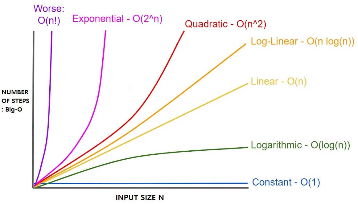
Meaning of different Time Complexity

Big-O	Known as
O(1)	Constant Time
O(log* N)	Iterative Logarithmic Time
O(logN)	Logarithmic Time
O(N)	Linear Time
O(N logN)	Log Linear Time
O(N^2)	Quadratic Time
O(N^p)	Polynomial Time
O(c^N)	Exponential Time
O(N!)	Factorial Time

Following is the visualization of some of the above notations:

Some points:

• The target is to achieve the lowest possible time complexity for solving a problem.

• For some problems, we need to good through all element to determine the answer. In such cases, the minimum Time Complexity is O(N) as this is the read to read the input data.

• For some problems, theoretical minimum time complexity is not proved or known. For example, for Multiplication, it is believed that the minimum time complexity is O(N logN) but it is not proved. Moreover, the algorithm with this time complexity has been developed in 2019.

• If a problem has only exponential time algorithm, the approach to be taken is to use approximate algorithms. Approximate algorithms are algorithms that get an answer close to the actual answer (not but exact) at a better time complexity (usually polynomial time).

• Several real world problems have only exponential time algorithms so approximate time algorithms are used in practice. One such problem is Travelling Salesman Problem. Such problems are NP-hard.

Brief Background on NP and P

Computation problems are classified into different complexity classes based on the minimum time complexity required to solve the problem.

Different complexity classes include:

• P (Polynomial)

• NP (Non-polynomial)

• NP-Hard

• NP-Complete

• P:

The class of problems that have polynomial-time deterministic algorithms (solvable in a reasonable amount of time).
P is the Set of problems that can be solved in polynomial time.

• NP:

The class of problems that are solvable in polynomial time on a non-deterministic algorithms.
Set of problems for which a solution can be verified in polynomial time.

• P VS NP

If the solution to a problem is easy to check for correctness, must the problem be easy to solve?
P is subset of NP. Any problem that can be solved by deterministic machine in polynomial time can also be solved by non-deterministic machine in polynomial time.

• NP - HARD
  Problems that are "at least as hard as the hardest problems in NP".

• NP-complete
  Problems for which the correctness of each solution can be verified quickly and a brute-force search algorithm can actually find a solution by trying all possible solutions.

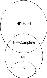
Relation between P and NP:

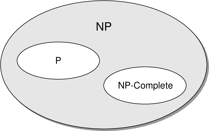
P is contained in NP.
NP complete belongs to NP
NP complete and P are exclusive

One of the biggest unsolved problems in Computing is to prove if the complexity class P is same as NP or not.

P = NP or P != NP

If P = NP, then it means all difficult problems can be solved in polynomial time.

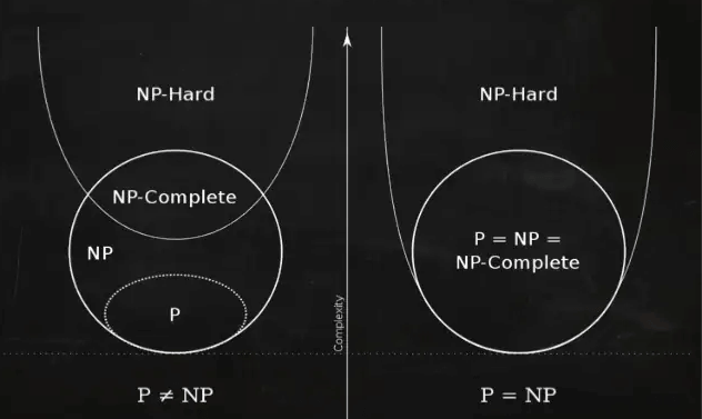
There are techniques to determine if a problem belongs to NP or not. In short, all problems in NP are related and if one problem is solved in polynomial time, all problems will be solved.

With this article at OpenGenus, you must have a strong idea of Time Complexity, Complexity classes and different notations. Enjoy.