
In this article, we have explored the concept of Amortized Time Complexity by taking an example and compared it with a related concept: Average Case Time Complexity.
| Table of Contents |
|---|
| 1)Glance of Time Complexity |
| 2)Introduction |
| 3)Amortized vs Average |
| 4)Understanding amortization using Dynamic Array |
| 5)Analysing Worst Case Complexity |
| 6)Analysing Amortized Complexity |
| 7)Conclusion |
Pre-requisite:
1) Glance of Time Complexity
Let's first go through the concept of time complexity.
Time complexity is the measure of time that a particular algorithm takes to complete its execution.It is measured as a function of the algorithm's input size.The time complexity doesn't indicate the exact execution time of an algorithm rather it gives an idea of variation of time with corresponding variation of input size.
There are three types of notations in which the complexity can be represented:
1.Big Oh notation(O):It is used to indicate the upper bound or the worst case time complexity of an algorithm.
2.Big Theta notation(θ): It is used to indicate the complexity for an algorithm averaged over all possible inputs.
3.Big Omega notation(Ω): It is used to indicate the lower bound or the best case time complexity of an algorithm.
Let's understand the above cases with the help of Linear Search algorithm
Let n be size of the array.
1)Worst Case Complexity: It occurs when the search element is found at the last position in the array or not found in the array.It requires n comparisions in such cases.
Hence, the worst case time complexity of Linear Search algorithm is O(n).
2)Average Case Complexity: In Linear Search the number of cases of searching is n+1
(considering extra case when element is not found in the array).
Average case works on probability.
Let T1, T2, T3,....., Tn be the time complexities and P1, P2, P3,....., Pn be the probabilities for all the possible inputs.
The above equation gives the average time complexity.
In linear search,let the probability for finding an element at each location be the same i.e., 1/n (as we have n locations)
For first element we perform 1 comparision,
For second element we perform 2 comparisions,
For third element we perform 3 comparisions,...and so on.
Hence, the average case complexity for linear search is O(n).
The average case analysis is not easy to do in most cases and it is rarely done.
3)Best Case Complexity: It occurs when the search element is found at the first position in the array. It requires only one comparision in such case.
Hence, the best case complexity of Linear Search algorithm is Ω(1).
Apart from the above mentioned types of complexity representation, there is one more representation called Amortized Time Complexity which is rarely used.
2) Introduction to Amortized time complexity
Amortized time complexity is the "Expected Time Complexity" which is used to express time complexity in cases when an algorithm has expensive worst-case time complexity once in a while compared to the time complexity that occurs most of the times.
Another way of saying is Amortized complexity is used when algorithms have expensive operations that occur rarely.
3) Amortized vs Average Time Complexity
Though they seem to be similar there is a subtle difference.
Average case analysis relies on probabilistic assumptions about the data structures and operations in order to compute an expected running time of an algorithm.
In the above discussion of analysing average case complexity of Linear Search, we've assumed that the probability of finding an element at each location is same.
On the other hand, Amortized complexity takes into consideration the total performance of an algorithm over sequence of operations.
If amortized time complexity of an algorithm is O(f(n)) then individual operations may take more time than O(f(n)) but most of the operations take O(f(n)) time.
If average time complexity of an algorithm is O(g(n)) then individual operations may take more time than O(g(n)) but at random the operations take O(g(n)) time.
4) Understanding amortization using Dynamic Array
Dynamic Array is the best example to understand Amortized Time complexity.
Dynamic array is a linear data structure which is growable and shrinkable in size upon necessity.
vector in C++ and ArrayList in Java use the concept of Dynamic array in their implementation.
There arises two cases for insertion in dynamic array:
1.When there exists free space in the array
Time complexity here is O(1).
2.When there is no space, a new array is to be created of size double the original array,the elements in the original array are to be copied and new element is inserted.
Time complexity here is
(Creation of new array of double the original size)+(Copying the elements of the original array)+(Insertion of the new element)
O(2N)+O(N)+O(1)=O(3N+1) where N is the size of the original array.
5) Analysing Worst Case Complexity
Suppose that we are doing insertion operation on the array for N times where N is the size of the array.In the worst case each operation takes O(3N) time complexity
Time complexity for overall operation is N×O(3N)=O(3N2)
Ignoring constant,
The worst case time complexity for N insertions is O(N2)
Now, let's analyse amortized time complexity.
6) Analysing Amortized Complexity
The amortized analysis averages the running times of operations in a sequence.
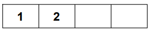
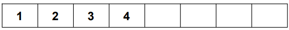
Assume initially size of the array is 1

Insert 1
Time: 1

Now, there is no space for insertion hence take an array of size double that of the original array i.e., 2
Copy the elements of the original array i.e., 1
Insert 2
Time: 2+1+1=4
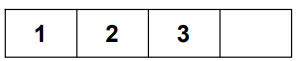
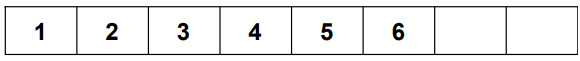
Now, there is no space for insertion hence take an array of size double that of the original array i.e., 4
Copy the elements of the original array i.e., 1,2
Insert 3
Time: 4+2+1=7
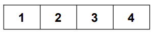
Insert 4
Time: 1
Now, there is no space for insertion hence take an array of size double that of the original array i.e., 8
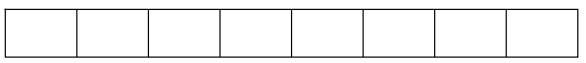
Copy the elements of the original array i.e., 1,2,3,4
Insert 5
Time: 8+4+1=13

Insert 6
Time: 1
Insert 7
Time: 1
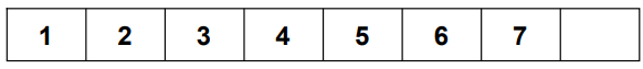
Insert 8
Time: 1
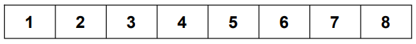
and so on...
Assume there would be m appends.
Hence the cost of m appends would be m since we are appending m elements(the append operation would cost O(1)) plus the cost of doubling when the array needs to grow.
Let's calculate the cost for doubling of array
The first doubling costs 1,second doubling costs 2,third doubling costs 4...and so on.
It's easier to solve the above equation if we reverse it.
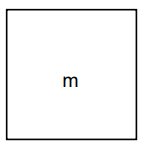
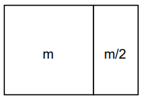
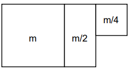
Adding m
Adding m/2
Adding m/4
Adding m/8
and so on...
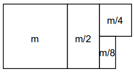
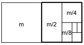
The highlighted box equals to m summing the total to 2m.
Hence keeping everything together appends cost m and doubling costs 2m.
Hence the total sum would be 3m i.e., O(m) .
Therefore m appends costs O(m). So each append costs O(1).
This is amortized complexity for dynamic array.
7) Conclusion
Though the amortized complexity for an append is O(1), the worst case it takes is still O(n) where n is size of the array. Therefore, with this article at OpenGenus, you must have a solid idea of Amortized time complexity.