In this post, we discuss interpolation search algorithm, its best, average and worst case time complexity and compare it with its counterpart search algorithms. We derive the average case Time Complexity of O(loglogN) as well.

Table of contents:

1. Basics of Interpolation Search
2. Time Complexity Analysis
3. Best Case Time Complexity
4. Average Case Time Complexity
5. Difference between an log(n) and log(log(n)) time compexity
6. Worst Case Time Complexity

Prerequisite: Interpolation Search, Binary Search

Basics of Interpolation Search

Interpolation Search is a search algorithm used for searching for a key in a dataset with uniform distribution of its values. An improved binary search for sorted and equally distributed data.

Uniform distribution means that the probability of a randomly chosen key being in a particular range is equal to it being in any other range of the same length. Therefore we expect to find target element at approximately the slot determined by the probing formula which we shall discuss below.

Comparison with binary search

Binary search chooses the middle element of the search space discarding a half sized chunk of the list depending on the comparison made at each iteration.
Interpolation search goes through different locations according to the search key, meaning it only requires the order of the elements, search space is reduced to the part before or after the estimated position at each iteration.

At each search step, the algorithm will calculate the remaining search space where the target element might be based on the low and high values of the search space and target value.

A comparison is made between the target and the value found at this position, if it is not equal then the search space is reduced to the part before or after the estimated position

The probing formula used is described below;

position(mid) = low + ((target – arr[low]) * (high – low) / (arr[high] – arr[low]))

This formula returns a higher value pos(mid) when target is closer to arr[high] and smaller value of pos(mid) when target is closer to arr[low].

An example

Given a dataset of 15 elements [10, 12, 13, 16, 18, 19, 20, 21, 22, 23, 24, 33, 35, 42, 47] and a target of 18. The algorithm will find the target in two iterations.

1st Iteration:

• mid = 0 + 8 * $\frac{13}{37}$ -> 3
• arr[3] = 16 < 18, therefore mid + 1 = 4

After this first step the search space is reduced, we know the target lies between index 3+1 to last index.

2nd Iteration:

• mid = 4 + 0 * $\frac{9}{29}$ -> 4
• arr[4] = 18 == target, terminate and return mid.

Algorithm

1. Calculate the value of pos(mid) using the probing formula and start search from there.
2. If the pos value is equal to target, return index of value and terminate.
3. If it does not match, probe position to find new mid using probing formula.
4. If value is greater than arr[pos] search the higher sub-array, right sub-array.
5. If value is greater than arr[pos] search the lower sub-array, left sub-array.
6. Repeat until the target is found, terminate when the sub-array reduces to zero.

Code

#include<iostream>
#include<vector>

using std::vector;
using std::cout;
using std::endl;

class InterPolationSearch{
    private:
        int probePosition(vector<int> arr, int target, int low, int high){
            return (low + ((target - arr[low]) * (high - low) / (arr[high] - arr[low])));
        }
    public:
        int search(vector<int> arr, int target){
            int n = arr.size();

            if(n == 0)
                return -1;

            //search space
            int low = 0, high = n - 1, mid;

            while(arr[high] != arr[low] && target >= arr[low] && target <= arr[high]){
                mid = probePosition(arr, target, low, high);
                
                if(target == arr[mid])
                    return mid;
                else if(target < arr[mid])
                    high = mid - 1;
                else
                    low = mid + 1;
            }
            return -1;
        }
};

int main(){
    InterPolationSearch ips;
    vector<int> arr = {10, 12, 13, 16, 18, 19, 20, 21,
                 22, 23, 24, 33, 35, 42, 47};
    int target = 18;
    cout << ips.search(arr, target) << endl;
    return 0;
}

Output:

//index of 18 in list
Output: 4

Time Complexity Analysis

The time complexity of this algorithm is directly related to the number of times we execute the search loop because each time we execute the body of the while loop we trigger a probe(comparison) on an element in the list.

Best Case Time Complexity

In the best case we assume that we find the target in just 1 probe making a constant time complexity O(1).

Average Case Time Complexity

Lemma: Assuming keys are drawn independently from a uniform distribution then the expected number of probes C is bound by a constant.
Proof: We assume that the current search space is from o - n-1 and keys $x_i$ are independently drawn from a uniform distribution.
The probability of a key to be less than or equal to y is $p=\frac{y-arr\left[0\right]}{arr[n-1]-arr\left[0\right]}$.
Generally the probability of exactly i keys being less than or equal to y is $\left(\left(\begin{array}{c}n\\ i\end{array}\right)\right)p^i(1-p{)}^{n-i}$.

And because the distribution is binomial we expect $\mu =np$ and variance ${\sigma }^2=np(1-p)$ .

To determine C we do the following;
$C=\sum _{i=1}^{\infty }i·pr\left[exactly i probes are used\right]=\sum _{i=1}^{\infty }·pr\left[at least i probes are used\right]$

Observation let f(x)=x(1-x) therefore $f\left(x\right)\le \frac{1}{4}$ holds for all $x\in \mathbb{R}$.

Proof: f(x) is quadratic with the maximum at x = 1/2 and value f(1/2)=1/4, that is:

$\frac{d}{dp}p\left(1-p\right)=\frac{d}{dp}p-p^2=1-2p=0\leftrightarrow p=\frac{1}{2} and \frac{d^2}{d{p}^2}p\left(1-p\right)=-2<0$.

By the above observation we have ${\sigma }^2=p(1-p)n\le \frac{1}{4}n$ and therefore
$c\le 2+\sum _{i=3}^{\infty }\frac{{\sigma }^2}{(\left(i-2\right)ceil\left(\sqrt{n}\right){)}^2}$

Which simplifies to $2+\frac{1}{4}\frac{{\pi }^2}{6}\le 2.42$.

With that we can start to prove the log(log(n)) time complexity for the average case.

Let T(n) be the average number of probes needed to find a key in an array of size n.
Let C be the expected number of probes needed to reduce the search space of size x to $\sqrt{x}$.

According to the lemma C will be bound by a constant $C\text{'}$.
Therefore we have the following equation, $T\left(n\right)\le C\text{'}+T\left(\sqrt{n}\right)$.

To eliminate $T\left(\sqrt{n}\right)$.

Assume that $n={z^2}^k$ for some k, $z\in \mathbb{N}$ and T(z) is small.

We have the following equation;
$T\left(n\right)=T\left({z^2}^k\right)\le C\text{'}+T\left({z^2}^{k-1}\right)\le C\text{'}+C\text{'}+T\left({z^2}^{k-2}\right)\le C\text{'}+C\text{'}+...+C\text{'}+T\left(z\right)=kC\text{'}+T\left(z\right)$

And because $n={z^2}^k$ and $z\ge 2$ if n > 1, ${\log }_2\left(z\right)\ge 1$.

Therefore, $k={\log }_z\left({\log }_2\right(n\left)\right)=\frac{{\log }_2\left({\log }_2\right(n\left)\right)}{{\log }_2\left(z\right)}\le {\log }_2\left({\log }_2\right(n\left)\right)$

In conclusion $T\left(n\right)\le C\text{'}\times log\left(log\right(n\left)\right)+T\left(z\right)$.

And after ingoring T(z) and using the constant from the lemma described we have
T(n) <= 2.42 * log(log(n)) .

Therefore for the average case we have O(log(log(n)) time complexity.

Difference between an log(n) and log(log(n)) time compexity

log(n) cuts input size by some constant factor say 2, after every iteration therefore the algorithm will terminate after log(n) iterations when the problem size hah been shrinked down to 1 or 0.

log(log(n)) cuts the input by a square root at each step.

An example.

Given an input size of 256.

log(n) will have 8 iterations that is $2^8$. The problem will be halved at each step.

log(log(n)) will have 3 iterations because at each step the problem is square rooted, 256, 16, 4, 2

In summary, the number of iterations by interpolation search algorithm will be less than half the number of iterations of the binary search if the list has a uniform distribution of elements and is sorted.

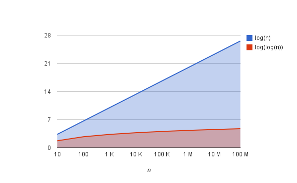
Note: If n is 1 billion, log(log(n)) is about 5, log(n) is about 30.

Worst Case Time Complexity

In the worst case, it makes n comparisons. This happens when the numerical values of the targets increase exponentially.

An Example:

Given the array [1, 2, 3, 4, 5, 6, 7, 8, 9, 100] and target is 10, mid would be repeatedly set to low and target would be compared with every other element in the list. The algorithm degrades to a linear search time complexity of O(n) .
We can improve this complexity to O(log(n)) time if we run interpolation search parallelly with binary search, (binary interpolation search), this is discussed in the paper in the link at the end of this post.

Space complexity is constant O(1) as we only need to store indices for the search in the list.

Question

Can you think of applications of this algorithm? Hint: An ordered dataset with uniform distribution.