In this article, we have taken an in-depth look at the operations or algorithms that have a constant time in terms of asymptotic notation of time complexities. Is O(1) really a practical way of representing the time complexity of certain algorithms/ operations?

Table of content:

1. Getting started with the Memory model
2. Let's talk about O(1)
3. Digging deep into access time
4. Testing our claim
5. Conclusions
   5.1 Physical analysis
   5.2 Analysis of algorithms

Let's find out!

1. Getting started with the Memory model

1.1 Random Access Machine (RAM) and External Memory Model

Let's talk about the Random Access Machine first, i.e., the RAM. A RAM physically consists of a central processing unit (CPU) and a memory. The memory itself has various cells inside it that are indexed by means of positive integers. A cell is capable of holding a bit-string. Talking about the CPU, it has a finite number of registers (an accumulator and an address register, to be specific).

In a single step, a RAM can either perform an operation (simple arithmetic or boolean operations) on its registers or access memory. When a portion of the memory is accessed, the content of the memory cell indexed by the content of the address register is either loaded into the accumulator or is directly written from the accumulator.

In this case, two timing models are used which are:

• The unit-cost RAM in which each operation has cost one, and the length of the bit-strings that can be stored in the memory cells and registers is bounded by the logarithm of the size of the input.

• The logarithmic-cost RAM in which the cost of an operation is equal to the sum of the lengths (bits) of the operands, and the contents of memory cells and registers don't have any specific constraints.

Now that you have an idea about the RAM, let's talk about the External Memory Model. An EM machine is basically a RAM that has two levels of memory. Getting into the specifics, the levels are referred to as cache and main memory or memory and disk, respectively. The CPU operates on the data that present in the cache. Both cache and main memory are each divided into blocks of B cells, and the data is transferred between them in blocks. The cache has size M and hence consists of M/B blocks whereas the main memory is infinite in size. The analysis of algorithms in the EM-model actually bounds the number of CPU steps and the number of block transfers. The time taken for a block transfer to be completed is equal to the time taken by Θ(B) CPU steps. In this case, the hidden constant factor is significantly large, and this is why the number of block transfers are taken into consideration in the analysis.

1.2 Levels/Hierarchy of Memory

The CPU cache memory is divided into three levels. The division is done by taking the speed and size into consideration.

• L1 cache: The L1 (Level 1) cache is considered the fastest memory that is present in a computer system.
  The L1 cache is generally divided into two sections:

1> The instruction cache: Handles the information about the operation that the CPU must perform.
2> The data cache: Holds the data on which the operation is to be performed.
The L1 cache is usually 100 times faster than the system RAM.

• L2 cache: The L2 (Level 2) cache is usually slower than the L1 cache, but has the upper hand in terms of size. The size of the L2 cache depends on the CPU, but generally it is in the range of 256kB to 8MB. It is usually 25 times faster than the system RAM.

• L3 cache: The L3 (Level 3) is the largest but also the slowest cache memory unit. Modern CPUs include the L3 cache on the CPU itself. The L3 cache is also faster than the system RAM, although it is not very significant.

1.3 Virtual Memory

Virtual memory is a section of the volatile memory that is created temporarily on the storage drive for the purpose of handling concurrent processes and to compensate for the high RAM usage.

Usually, virtual memory is considerably slower than the main memory because of the fact that the processing power is being consumed by the transportation of data instead of the execution of instructions. A rise in latency is also observed when a system needs to use virtual memory.

1.4 Virtual Address Translation (VAT) Model

The Virtual Address Translation (VAT) machines are RAM machines that use virtual addresses and also account for the cost of address translations and it has to be taken into consideration as well during the analysis of various algorithms.

For the purpose of understanding and demonstration, let us assume that:

P = Page size (P = 2ᵖ)
K = Arity of translation tree (K = 2ᵏ)
d = Depth of translation tree (dlogₖ(max used virtual address))
W = Size of the TC cache
τ = Cost of a cache fault (number of RAM instructions)

Both the physical and virtual addresses are strings in {0, K-1}ᵈ{0,...,P-1}. Such strings correspond to a number present in the interval [0, KᵈP-1] in a natural manner. The {0, K-1}ᵈ part of the address is the index and is of length d which is an execution parameter that is fixed prior to the execution. It is also assumed that d = [logₖ(maximum used virtual address/P)]. The {0,...,P-1} part of the address is called the page offset where P is the page size (as specified before).

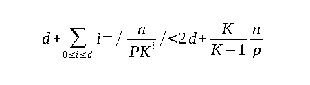
Coming to the actual translation process, it is basically a tree walk/traversal. We have a K-ary tree T of height d. The nodes of the tree are the pairs (l, i) where l >= 0 and i >= 0. Here l is the layer of the node and i is the total number of nodes itself. The leaves of the tree are present on layer zero and a node (l, i) on layer l >= 1 has K children on the layer l-1. In particular, the node (d, 0), the root, has children (d-1, 0),...,(d-1, K-1). The leaves of the tree are the physical pages of the main memory of a RAM machine. For example, to translate the virtual address xₔ₋₁...x₀y, we will start from the root of T and then follow the path which will be described by xₔ₋₁...x₀. This path is referred to as the translation path for the address and it ends in the leaf (0, Σ₀≤ᵢ≤ₔ₋₁xᵢKᶦ).

The following figure depicts the process in a generic way:

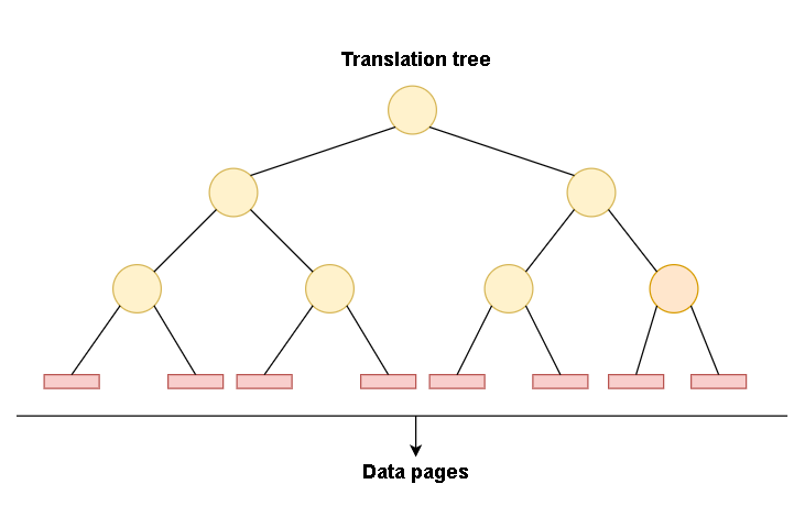
We come to the conclusion:

If D and i are integers such that D >= 0 and i >= 0, the translation paths for addresses i and i+D differ in at least the max(0, logₖ(D/P)) nodes.

1.5 Translation costs and Cache faults

In a research that was conducted earlier, six simple programs were timed for different inputs, namely, permuting the elements of an array of size n, random scan of an array of size n, n random binary searches in an array of size n, heap sort of n elements, introsort (hybrid of quick sort, heap sort and insertion sort) of n elements and sequential scan of an array of size n. It was found that for some of the programs, the measured running time coincided with the original predictions of the models. However, it was also found that the running of random scan seems to grow as O(nlog²n), and that doesn't really coincide with the original predictions of the models.

You might be wondering as to why are the predicted and the measured run times different? We will have to do some digging in order for us to understand that. Modern computers have virtual memories and each individual process has its own virtual address space. Whenever a process accesses memory, the virtual address has to be translated into a physical address (similar working as that of NAT, network address translation). This translation of virtual addresses into physical addresses isn't exactly trivial, and hence has a cost of its own. The translation process is usually implemented as a hardware-supported walk in a prefix tree and this tree is stored in the memory hierarchy and because of this, the translation process may also sustain cache faults. Cache faults are a type of page fault that occur when a program tries to reference a section of an open file that is not currently present in the physical memory. The frequency of cache faults is actually dependent upon the locality of the memory accesses (lesser local memory accesses result in more cache faults).

The depth of the translation tree is logarithmic in the size of an algorithm's address space and hence, in the worst case, all memory accesses may lead to a logarithmic number of cache faults during the translation process.

2. Let's talk about O(1)

We know that the time complexity for iterating through an array or a linked list is O(n), selection sort is O(n²), binary search is O(logn) and a lookup in a hash table is O(1).
However, in this article, we will try to prove that accessing memory is not a O(1) operation, instead it is a O(√n) operation. We will try to prove this through both theoretical and practical means and hopefully you will be convinced by our reasoning by the end of the article.

3. Digging deep into access time

Let us take an example. Try to relate this example with how memory access works in a working system. Suppose you run a big shop that deals with games. Your shop has a circular storage for games and you have placed the games in an orderly manner and you remember as to which game can be found in which drawer/place. A customer comes to your shop, and asks for game X. You know where X is placed in your shop. Now, what would be the time taken by you in order for you to grab and bring the game back to the customer? It would obviously be bounded by the distance that you have to walk to get that game, the worst case being when the game is present at either end of the shop, i.e., you will have to walk the full radius r.

Now let's take another example. Try to relate this example with how memory access works in a working system as well. Now let us suppose that you have upgraded your shop's infrastructure, and its storage capacity has increased tremendously. The radius of your shop is now twice times the original radius and hence the storage capacity has increased too. Now, in the case of the worst case scenario, you will have to walk twice the distance to retrieve a game. But we also have to think about the fact that the area of the shop is now doubled and therefore it can contain four times the original quantity of games.

From this relation, we can infer that N games that can fit into our shop storage is proportional to the square of the radius r of the shop.

Hence, N ∝ r²

Since we know that the time taken T to retrieve a game is proportional to the radius r of the shop, we can infer the following relation:

==> N ∝ T²
==> T∝√N
==> T = O(√N)

This scenario is roughly comparable to a CPU which has to retrieve a piece of memory from its library, which is the RAM.

The speed obviously differs significantly, but it is after all bounded by the speed of light.

In our example, we assumed that the storage space of our shop had a circular infrastructure. So how much data can be fitted within a specific distance r from the CPU?

What if the shape of the storage space was spherical? Well, in that case, the amount of memory that could be fitted within a radius r would then become proportional to r³.

However, in practice, computers are actually rather flat because of many factors such as form-factor, cooling issues, etc.

4. Testing our claim

Let's say that we have a program that iterates over a linked list of length N, consisting of about 64 to 400 million elements. Each node also contains a 64 bits pointer and 64 bits of dummy data. The nodes of the linked list are also jumbled around in memory such that the memory access for each node is random. We will be measuring iterating through the same list a few times, and then plotting the time taken per element. Well, if the access time really were O(1), then we would get a flat plot (in the graph).

However, interestingly, this is what we actually get:

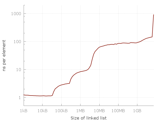
The graph plotted above is a log-log graph, and hence the differences that are visible in the figure are actually huge in size. In the figure, there is a noticeable spike or jump from about one nanosecond per element all the way up to a microsecond.

Now why is that happening? Try to recall what we spoke about in the Getting started with the Memory model section of this article. The answer to that question is caching. Off-chip or distant communication in RAM can be quite slow at times and in order to combat this con, the concept of cache was introduced. The cache basically is an on-chip storage that is much more faster and closer.

The system on which these tests were conducted had three levels of cache called L1, L2, L3 of 32 kiB, 256 kiB and 4 MiB each respectively with 8 GiB of RAM (with about 6GiB being free at the time of the experiment).

In the following figure, the vertical lines are represented by the cache sizes and the RAM:

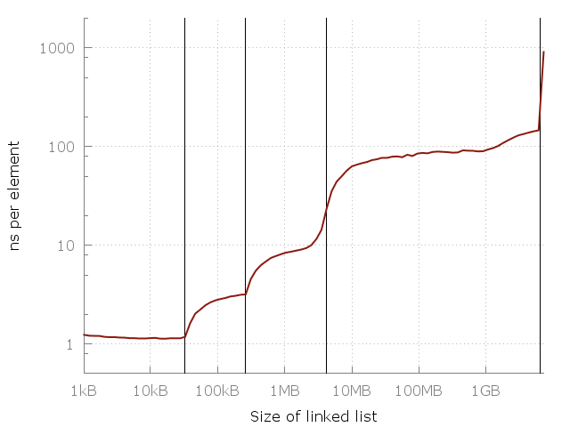
You might notice a pattern in the figure posted above. The importance and the role of caches also becomes very clear.

If you notice, you can see that there is a roughly a 10x slowdown between 10kB and 1MB. The same is true for the phase between 1MB and 100MB and for 100MB and 10Gb as well. It appears as if for each 100-fold increase in the usage of the memory, we get a 10-fold slowdown.

Let's compare that with our claim:

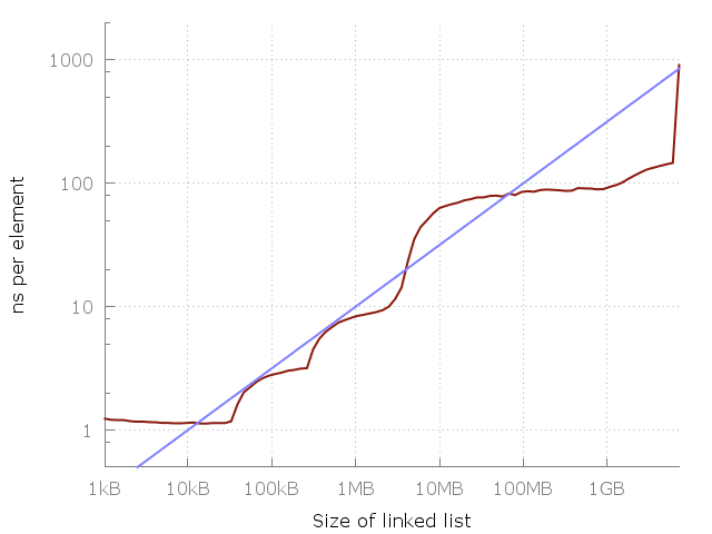
In the figure above, the blue line corresponds to a O(√N) cost each time the memory is accessed.

So, what happens when we reach the latter (right) side of the graph? Will there be a continuous rise in the graph or would it become flat?
It will actually flatten for a while until the memory could no longer be fit on the SSD and the help of the HDD is needed. From there, we would go to a disk server and then to a data-center, etc.

For each such jump, the graph would flatten for a while, but the rise will always arguably come back.

5. Conclusions

5.1 Physical analysis

The cost of a memory access depends upon the amount of memory that is actually being accessed as O(√N), where N = amount of memory being touched between each memory access.

From this, we can conclude that if one touches the same list/table in a repetitive manner, then iterating through a linked list will become a O(N√N) operation, the binary search algorithm will become a O(√N) operation and a hash map lookup will also become a O(√N) operation.

What we do between subsequent operations performed on a list/table also matters. If a program is periodically touching N amount of memory, then any one memory access should be O(√N).So if we are iterating over a list of size K, then it will be a O(K√N) operation. Now, if we iterate over it again (without accessing any other part of the memory first), it will become a O(K√K) operation.

In the case of an array (size K), the operation will be O(√N + K) because it is only the first memory access that is actually random. However, iterating over it again will become a O(K) operation.

That makes an array more suitable for scenarios where we already know that iteration has to be performed.

Hence, memory access patterns can be of significant importance.

5.2 Analysis of algorithms

Before proceeding with our conclusive remarks on certain algorithms, some assumptions that are necessary for the analysis to be meaningful have been written below.

1. Moving a single translation path to the translation cache costs more than a single instruction, but doesn't cost more than the instructions that are the equivalent to the size of a page. If at least one instruction is performed for each cell in a page, then the cost of translating the index of that page can be amortized, i.e., 1 <= τd <= P.
2. The fan-out of the translation tree is at least 2, i.e., K >= 2.
3. The translation tree suffices to translate all the addresses but is not significantly larger, i.e., m/P <= Kᵈ <= 2m/P. Because of this, we get log(m/P) <= dlogK = dk <= log(2m/P) = 1 + log(m/P). In turn, we have logₖ(m/P) <= d <= logₖ(2m/P) = (1 + log(m/P)) / k.
4. The translation cache is capable of holding at least one translation path, but it is still significantly smaller than the main memory, i.e., d <= W < m^Θ where Θ ∈ (0, 1).

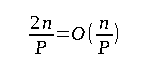
• Sequential access: Let's suppose that we have an array of size n. If b is the base address of an array, then we need to translate addresses in the order b, b+1, b+2,...., b+n-1. For P consecutive accesses, the translation path is going to stay constant, and so at most 2n/P indices must be translated for a total cost of at most τd(2+n/P). Referring to our first assumption, this would translate to at most τd(n/P + 2) <= n + 2P.

The analysis can be improved significantly by keeping the current translation path in the cache and hence limiting the first translation's faults to at most d. The translation path changes after every Pᵗʰ access. A change is observed in this case at most a total of ⌈n/P⌉ times. Whenever the path does undergo a change, the last node will also change as well. The node that is present next to the last node also changes after every Kᵗʰ change of the last node and hence changes at most ⌈n/(PK)⌉ times.

Hence, in total, we incur:

The cost is bounded by 2τd + 2τn/P <= 2P + 2n/d, which is asymptotically smaller than the RAM complexity.

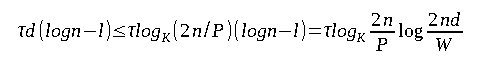
• Random access: In random access, the worst case occurs when no node of any translation path is in the cache. The total translation cost in this case is bounded by τdn and is at most τnlogₖ(2n/P).

Let us assume that the translation cache satisfies the initial segment property for the purpose of the analysis of a lower bound. The translation path will end in a random leaf of the translation tree and for every leaf, some initial segment of the path that ends in this leaf will be cached. Let u be an uncached node of the translation tree of minimal depth, and let v be a cached node of the translation tree of maximal depth. If the depth v is larger than u by a margin of 2 or more, then it will be better to cache u instead of v. Hence, the expected length of the path cached is at most logₖW and the expected number of faults incurred during the translation would be d - logₖW.

Hence, the total expected cost is at least τnlogₖn/(PW) <= τn( - logₖW), which is asymptotically larger than the RAM complexity.

• Binary search: Let's assume that we have to perform n binary searches in an array of length n. Each search will search for a random element of the array. For the sake of simplicity, let us assume the n is a power of two minus one. Now we cache the translation path of the top l layers of the search tree and the translation path of the current node of our search. The top l layers contain 2ˡ⁺¹ - 1 vertices and so we need to store at most d2ˡ⁺¹ nodes of the translation tree. Keep in mind that this is only feasible if d2ˡ⁺¹ <= W.

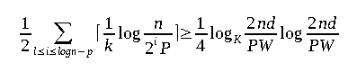
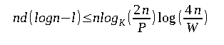
The remaining of the logn - l steps of the binary search causes at most d cache faults. Hence, the total cost per search will be bounded by:

The expected number of cache misses per search will be at least:

• Heapify and Heapsort: An array or a list (A[1...n]) storing elements from an ordered list is heap-ordered if A[i] <= A[2i] and A[i] <= A[2i+1] ∀ 1 <= i <= ⌊n/2⌋. An array can be transformed to a heap by calling operation sift(i) for i = ⌊n/2⌋ down to 1. This function repeatedly changes interchanges z = A[i] with the smaller of its two children until the heap property is satisfied. We will use the following translation replacement strategy.

The extremal translation (for n consecutive addresses, paths to the first and last address in the range) paths (2d-1 nodes), non-extremal (nodes that are not on the extremal path) paths of the translation paths for z address (a₀,...,a₂₋₁) and one additional translation path a∞ (⌊logₖ(n/P)⌋ nodes for each) are stored. The additional translation path is only required when z != logn. When this array is undergoing siftdown, for any element A[i], a₀ will be equal to the address of A[i], a₁ will be the address of one of the children of i (if A[i] is moved, then this is where will be moved), a₂ will the address of one of the grandchildren of i (in case is moved down two levels, it will be moved here), and so on. The additional translation path is only used for the addresses that are more than z levels below the level containing i.

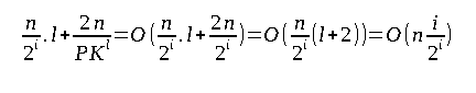
Let's place an upper bound on the number of the translation cache misses. Preparing the extremal paths can cause up to 2d + 1 misses. Now we have to consider the translation cost for aᵢ, 0 <= i <= z-1. In the case of aᵢ, n/2ᶦ unique values are assumed. On the assumption that the siblings in the heap always lie in the same page, the index if each aᵢ will decrease over time, and hence the total number of translation cache misses will be bound to the number of non-extremal nodes in range. We obtain the following bound in terms of translation cache misses:

If p + (l-1)k < i <= p + lk, where l >= 1 and i <= z-1, we can use x = n/2ᶦ and obtain a bound in terms of translation cache misses of at most:

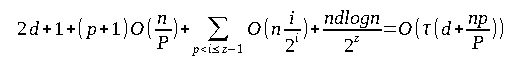
Now, there are a total of n/2ᶻ siftdowns in layers z and above, and they use the additional translation path. For each such siftdown, we only need to translate logn addresses and each such translation will cause less than d misses. The total will be lesser than n(logn)d/2ᵃ. We get:

Next, we can prove the lower bound by assuming that W < n/2P.

The addresses will start being swept a₀, then a₁, and so on. No other accesses occur in the sub-array during this time. Hence, if the Least Recently Used (LRU) strategy is used, there will be at least pn/(2P) translation cache misses to the lowest level of the translation tree. This will give us the Ω(np/P) part of the lower bound and so the total cost will be Ω(τ(d + np/P)).

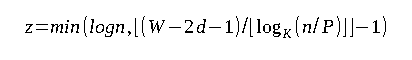
Coming to the sorting phase of heapsort, the element that is stored in the root is repeatedly removed and moved to the rightmost leaf to the root, after which the siftdown process occurs to restore its heap property. The siftdown will start in the root and after accessing the address i of the heap, it moves to the address 2i or 2i+1. For analysis purposes, let us assume that the data cache and the translation cache are same in terms of size, i.e., W = M. The top l layers of the heap will be stored in the data cache and the translation paths to the vertices to these layers will be stored in the translation cache, where 2ˡ⁺¹ < M. Each of the remaing logn - l siftdown steps might cause d cache misses. The total number of cache faults will hence be bounded by:

With this article at OpenGenus, you must have a deep idea of Time Complexity.

6. References

• "On a Model of Virtual Address Translation" by Tomasz Jurkiewicz and Kurt Mehlhorn from Max Planck Institute for Informatics, Germany: PDF