
In this article, we have explored the architecture of a Densely Connected CNN (DenseNet-121) and how it differs from that of a standard CNN. An overview of CNNs and its basic operations can be found here.
Table of content:
- Introduction to DenseNet
- DenseNet Architecture & Components
- DenseNet-121 Architecture
- Conclusion
In short, DenseNet-121 has the following layers:
- 1 7x7 Convolution
- 58 3x3 Convolution
- 61 1x1 Convolution
- 4 AvgPool
- 1 Fully Connected Layer
We will dive deeper.
Introduction to DenseNet
In a traditional feed-forward Convolutional Neural Network (CNN), each convolutional layer except the first one (which takes in the input), receives the output of the previous convolutional layer and produces an output feature map that is then passed on to the next convolutional layer. Therefore, for 'L' layers, there are 'L' direct connections; one between each layer and the next layer.

However, as the number of layers in the CNN increase, i.e. as they get deeper, the 'vanishing gradient' problem arises. This means that as the path for information from the input to the output layers increases, it can cause certain information to 'vanish' or get lost which reduces the ability of the network to train effectively.
DenseNets resolve this problem by modifying the standard CNN architecture and simplifying the connectivity pattern between layers. In a DenseNet architecture, each layer is connected directly with every other layer, hence the name Densely Connected Convolutional Network. For 'L' layers, there are L(L+1)/2 direct connections.

DenseNet Architecture & Components
Components of DenseNet include:
- Connectivity
- DenseBlocks
- Growth Rate
- Bottleneck layers
Connectivity
In each layer, the feature maps of all the previous layers are not summed, but concatenated and used as inputs. Consequently, DenseNets require fewer parameters than an equivalent traditional CNN, and this allows for feature reuse as redundant feature maps are discarded. So, the lth layer receives the feature-maps of all preceding layers, x0,...,xl-1, as input:
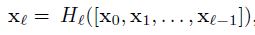
where [x0,x1,...,xl-1] is the concatenation of the feature-maps, i.e. the output produced in all the layers preceding l (0,...,l-1). The multiple inputs of Hl are concatenated into a single tensor to ease implementation.
DenseBlocks
The use of the concatenation operation is not feasible when the size of feature maps changes. However, an essential part of CNNs is the down-sampling of layers which reduces the size of feature-maps through dimensionality reduction to gain higher computation speeds.
To enable this, DenseNets are divided into DenseBlocks, where the dimensions of the feature maps remains constant within a block, but the number of filters between them is changed. The layers between the blocks are called Transition Layers which reduce the the number of channels to half of that of the existing channels.
For each layer, from the equation above, Hl is defined as a composite function which applies three consecutive operations: batch normalization (BN), a rectified linear unit (ReLU) and a convolution (Conv).
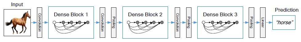
In the above image, a deep DenseNet with three dense blocks is shown. The layers between two adjacent blocks are the transition layers which perform downsampling (i.e. change the size of the feature-maps) via convolution and pooling operations, whilst within the dense block the size of the feature maps is the same to enable feature concatenation.
Growth Rate
One can think of the features as a global state of the network. The size of the feature map grows after a pass through each dense layer with each layer adding 'K' features on top of the global state (existing features). This parameter 'K' is referred to as the growth rate of the network, which regulates the amount of information added in each layer of the network. If each function H l produces k feature maps, then the lth layer has
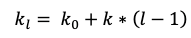
input feature-maps, where k0 is the number of channels in the input layer. Unlike existing network architectures, DenseNets can have very narrow layers.
Bottleneck layers
Although each layer only produces k output feature-maps, the number of inputs can be quite high, especially for further layers. Thus, a 1x1 convolution layer can be introduced as a bottleneck layer before each 3x3 convolution to improve the efficiency and speed of computations.
DenseNet-121 Architecture

A summarization of the various architectures implemented for the ImageNet database have been provided in the table above. Stride is the number of pixels shifts over the input matrix. A stride of 'n' (default value being 1), indicates that the filters are moved 'n' pixels at a time.
Using the DenseNet-121 architecture to understand the table, we can see that every dense block has varying number of layers (repetitions) featuring two convolutions each; a 1x1 sized kernel as the bottleneck layer and 3x3 kernel to perform the convolution operation.
Also, each transition layer has a 1x1 convolutional layer and a 2x2 average pooling layer with a stride of 2. Thus, the layers present are as follows:
- Basic convolution layer with 64 filters of size 7X7 and a stride of 2
- Basic pooling layer with 3x3 max pooling and a stride of 2
- Dense Block 1 with 2 convolutions repeated 6 times
- Transition layer 1 (1 Conv + 1 AvgPool)
- Dense Block 2 with 2 convolutions repeated 12 times
- Transition layer 2 (1 Conv + 1 AvgPool)
- Dense Block 3 with 2 convolutions repeated 24 times
- Transition layer 3 (1 Conv + 1 AvgPool)
- Dense Block 4 with 2 convolutions repeated 16 times
- Global Average Pooling layer- accepts all the feature maps of the network to perform classification
- Output layer
Therefore, DenseNet-121 has the following layers:
- 1 7x7 Convolution
- 58 3x3 Convolution
- 61 1x1 Convolution
- 4 AvgPool
- 1 Fully Connected Layer
In short, DenseNet-121 has 120 Convolutions and 4 AvgPool.
All layers i.e. those within the same dense block and transition layers, spread their weights over multiple inputs which allows deeper layers to use features extracted early on.
Since transition layers outputs many redundant features, the layers in the second and third dense block assign the least weights to the output of the transition layers.
Also, even though the weights of the entire dense block are used by the final layers, there still may be more high level features generated deeper into the model as there seemed to be a higher concentration towards final feature maps in experiments.
Conclusion
As DenseNets require fewer parameters and allow feature reuse, they result in more compact models and have achieved state-of-the-art performances and better results across competitive datasets, as compared to their standard CNN or ResNet counterparts.
We hope this article at OpenGenus proved useful to you in learning about the DenseNet architecture:)
References
- G. Huang, Z. Liu, van, and Weinberger, Kilian Q, “Densely Connected Convolutional Networks,” arXiv.org, 2016. arxiv.org/abs/1608.06993.