Guide to "An embarrassingly simple approach to Zero-Shot Learning"

Reading time: 35 minutes | Coding time: 20 minutes

In this article at OpenGenus, we will be discussing about "An embarrassingly simple approach to Zero-Shot learning" and go into details how to apply this approach that in a single line of code outperforms the state-of-art models. This has been formulated by Bernardino Romera-Paredes and Philip H. S. Torr from University of Oxford.

Basics

First, let's review the basic idea of zero-shot learning that we learned in this.

• Shot: The number of samples of a class you need in your data for the machine to learn about that class.

• Zero-shot learning is a method that helps us in predicting for a category which has zero shots(samples) in the dataset.

• The problems with classical approach is when new set of categories appear after learning we would have to add it to our model for training.

• We are always dependent on labelled data.

• We can easily identify a new object by having its description or using similarities of previously learned objects without actually needing data for those new objects.

• It is the learning of new concepts just by having a description of them with previously learned concepts. There are 2 stages in this process: Training and Inference.

• Many attempts have been made to exploit the discriminative capacity of attributes but cannot control the uncertainty of attribute prediction obtained from the Training stage.

An embarrassingly simple approach to ZSL has addressed the problem of auto classification in terms of computer vision and document classification.

Now, we will talk about in depth about a technique used in "An embarrassingly simple approach to ZSL"

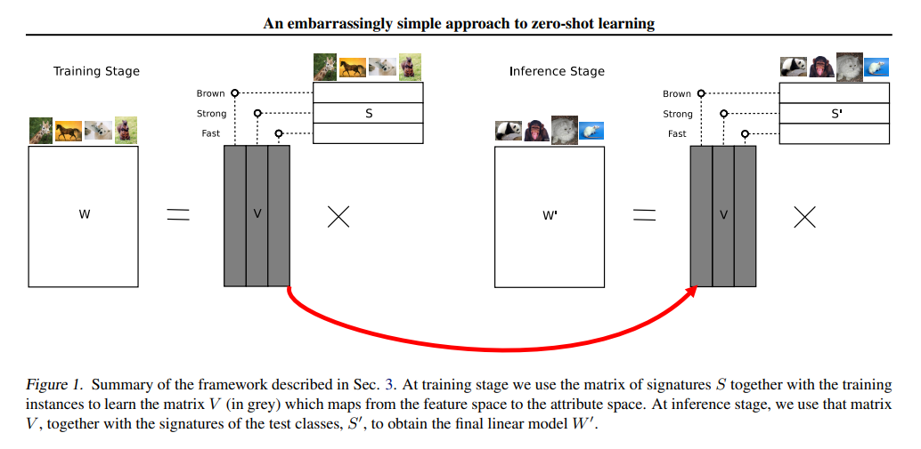
• The framework described with this approach is that of 2 layers which is built upon creating relationships between features, attributes and classes with the help of a linear model.

• The first layer helps in defining the relationship between features and attributes with the help of weights in that layer.

• The second layer deals with modelling the relationship between attributes and classes where the prescribed attribute signatures is fixed.

]

With matrix factorization, we can decompose a nxm matrix into Nxa and axM matrices where n is the number of features, m is the number of classes and a is the number of soft attributes.

Now what they do in the training stage is that they train nxm weight by co-efficient matrix and a signature matrix axm in an unsupervised manner.

• The transpose of input vector is multiplied with weight matrix in order to obtain the predicted class.

• For example, when classes are: Giraffe and Horse and the attributes are 'has_stripes', 'can_ride' and 'not_wild' then the signature matrix S would look something as below:

	Giraffe	Horse
has_stripes	1	0
can_ride	0	1
not_wild	1	1

• Now, we find nxa matrix V from the signature matrix and weight matrix W such that V . S = -W

• Once we are done with this, our aim is to predict for new classes so we build a signature matrix S' for them. Let's say our new classes are: Tigers and Zebras.

The new signature matrix S' can be described as:

	Zebra	Tiger
has_stripes	1	1
can_ride	0	0
not_wild	1	0

In order to predict for new classes, we first compute the dot product of V ( axm ) and the new signature matrix S'.

This will provide us with new weight matrix W'. For the new samples of tiger and zebra, we do argmax over the dot product of transpose of input vector x and -W'

That'll provide us with the prediction for new classes. This is the main approach to zero-shot learning with this technique.

Model Description

Let's first define some notations. There are z classes in the training stage where each of them have a signature composed of a attributes.

The signatures are represented in a signature matrix S consisting of boolean entries 0 and 1.

This helps in defining the soft link between attributes and classes. The instances available at training stage are denoted by X, where X belongs to R^(dxm) where d is the dimensionality of data and m is the number of instances.

Ground truth labels for each training instance belonging to one of the z classes is denoted by Y, where Y ∈ {-1,1}^(mxz)

Now, we can obtain ground truths for each instance just from Y and S.

If we were to learn a linear predictor by classical approach on this the we would have to optimize the loss function for output Y and dot product of transpose of X and W where W contains the parameters to be learned.

At the inference stage we want to distinguish between a new set of z' classes. To do so, we are provided with their attributes signatures, S' ∈ [0, 1]^(a×z').

Then, given a new instance, x, the prediction is given by argmax(transpose(X).V.Si') where V is given by W = V.transpose(S), V ∈ R^(dxa).

• In our demo, we are working with the famous MNIST dataset of digits.

• We need to partition the digits into seen and unseen classes from the machine. Label Encoder is used to encode target digits into values between 0 and number of classes - 1.

• After we have the encoded target values, weight matrix is made using logistic regression and attributes are created with unsupervised learning.

• The signature matrix is built with 2 components of each Principal Component Analysis (PCA) and Locally Linear Embedding (LLE).

• PCA: It is a technique for feature extraction where it combines input variables in such a way that we can drop the least important variables while still holding the important information by valuable variables.

This method of dimensionality reduction in PCA actually helps with avoiding overfitting the model.

• LLE: It is a lower-dimensional projection of the data which preserves distances within local neighborhoods.

• It can be thought of as a series of local Principal Component Analyses which are globally compared to find the best non-linear embedding.

• The signature matrix is built from the low dimensional important pca and lle components.

• New weight matrix is calculated from this signature matrix S and matrix V discussed earlier. From this, new predictions can be made about the unseen digits.

Demo

Let's start first with importing the libraries,

from sklearn import datasets, linear_model, preprocessing, decomposition, manifold
from sklearn.metrics import make_scorer, accuracy_score
import numpy as np
from sklearn.model_selection import cross_validate, cross_val_score, train_test_split

We are going to select some digits in our dataset of training and testing other with zero shot learning.

# Loading the MNIST dataset
X, y = datasets.load_digits().data, datasets.load_digits().target

# There are d dimensions, d=64
# z classes, z=6, [digit0, digit1, digit2, digit7, digit8, digit9]
lbl = preprocessing.LabelEncoder()
y_train = lbl.fit_transform(y[np.where((y == 0) | (y == 1) | (y == 2) | (y == 7) | (y == 8) | (y == 9))])
X_train = X[np.where((y == 0) | (y == 1) | (y == 2) | (y == 7) | (y == 8) | (y == 9))]

We first fit a logistic Regression model on the z classes mentioned for unsupervised learning.

model = linear_model.LogisticRegression(random_state=1)
model.fit(X_train, y_train)

Now, we calculate the signature matrix to find the new weight matrix for prediction during training stage.

# We have a attributes, a=4 [pca_d1, pca_d2, lle_d1, lle_d2]
# We have Signature matrix, S a x z
pca = decomposition.PCA(n_components=2)
lle = manifold.LocallyLinearEmbedding(n_components=2, random_state=1)
X_pca = pca.fit_transform(X_train)
X_lle = lle.fit_transform(X_train)

for i, ys in enumerate(np.unique(y_train)):
	if i == 0:
		S = np.r_[ np.mean(X_pca[y_train == ys], axis=0), np.mean(X_lle[y_train == ys], axis=0) ]
	else:
		S = np.c_[S, np.r_[ np.mean(X_pca[y_train == ys], axis=0), np.mean(X_lle[y_train == ys], axis=0) ]]

# From W and S calculate V, d x a
V = np.linalg.lstsq(S.T, W.T)[0].T

W_new = np.dot(S.T, V.T).T

print "%f"%np.sum(np.sqrt((W_new-W)**2))

# Predictions that happens in the training phase of zero shot learning
for ys, x in zip(y_train, X_train):
	print np.argmax(np.dot(x.T, W_new)), ys

40.152231
0 0
1 1
2 2
3 3
2 4
0 5
0 0
1 1
2 2
3 3
3 4
0 5
0 0
1 1
2 2
3 3
...

Here, we are going to describe the procedure in Inference stage. Firstly, we take test data as the digits which are not used in training i.e. 3, 4, 5 and 6.

Then we need to find the new signature matrix S' using the old pca and linear local embedding transformers
So we split the samples of digits 3, 4, 5 and 6 into data and output as their attributes: pca and lle(linear local embedding).

# INFERENCE
lbl = preprocessing.LabelEncoder()
y_test = lbl.fit_transform(y[np.where((y == 3) | (y == 4) | (y == 5) | (y == 6))])
X_test = X[np.where((y == 3) | (y == 4) | (y == 5) | (y == 6))]

# create S' (the Signature matrix for the new classes, using the old transformers)
X_test, X_sig, y_test, y_sig = train_test_split(X_test, y_test, test_size=4, random_state=1, stratify=y_test)

X_pca = pca.transform(X_sig)
X_lle = lle.transform(X_sig)

for i, ys in enumerate(np.unique(y_sig)):
	if i == 0:
		S = np.r_[ np.mean(X_pca[y_sig == ys], axis=0), np.mean(X_lle[y_sig == ys], axis=0) ]
	else:
		S = np.c_[S, np.r_[ np.mean(X_pca[y_sig == ys], axis=0), np.mean(X_lle[y_sig == ys], axis=0) ]]

As we have the new signature matrix S', we can find the new weight coefficient matrix.

# Calculate the new Weight/Coefficient matrix		
W_new = np.dot(S.T, V.T).T

Now, we use the argmax query over dot product for transpose of input vector x and new weight coefficient matrix as we discussed earlier to predict for the new unseen classes of digits.

# Check performance
correct = 0
for i, (ys, x) in enumerate(zip(y_test, X_test)):
		if np.argmax(np.dot(x.T, W_new)) == ys:
		correct +=1
		
print correct, i, correct / float(i)

286 722 0.396121883657

The accuracy of predicting the 4 unseen digits is 39.6% which is still better than random guessing accuracy of 25% and we get 286 samples correct out of 722.

Further reading:

• The original research paper: "An embarrassingly simple approach to Zero-Shot learning" by Bernardino Romera-Paredes and Philip H. S. Torr from University of Oxford.
• You can find the notebook for the code here

Enjoy this new knowledge in the fast growing field of Machine Learning.