In this article, we have presented the Architecture of YOLOv3 model along with the changes in YOLOv3 compared to YOLOv1 and YOLOv2, how YOLOv3 maintains its accuracy and much more.

Table of contents:

1. Introduction to Object Detection
2. Overview of YOLOv3
3. A walkthrough of YOLOv3 architecture
4. YOLOv3 high accuracy secret
5. What after YOLOv3?

Let us get started with Architecture of YOLOv3 model.

1. Introduction to Object Detection

In the field of computer vision, object detection is considered to be the most daunting challenges. There are multiple object detection algorithms but none of them created the buzz that YOLOv3 created. YOLO, or You Only Look Once, is considered to be the most popular object detection algorithms out there. Versions 1 to 3 of YOLO were created by Joseph Redmon and Ali Farhadi.

Back in 2016, the first version of YOLO was created and two years later, the popular YOLOv3 was implemented as an improved version of YOLO and YOLOv2. YOLO can be implemented using the Keras or OpenCV deep learning libraries.

Object detection models are used in Artificial Intelligence programs to perceive specific objects in a class as subjects of interest. The programs classifies the images into groups and puts similar looking images into one group. Other images are subsequently classified into various other classes.

But why the name “you only look once”? Well, it is because the convolutions used in predictions is based on a convolution layer that uses 1 x 1 convolutions.

2. Overview of YOLOv3

YOLO is a Convolutional Neural Network (CNN) used for real-time object detection. CNNs are classifier-based frameworks that interacts with input pictures as structured arrays of data and aims to recognize patterns between them (see picture beneath). YOLO enjoys the benefit of being a lot quicker than other object detection models while also maintaining accuracy.

It permits the model to view the entire image at test time, so its predictions are informed by the overall global context of the image. YOLO, as well as other CNN algorithms "score" the regions based on similarities present in images to the predefined classes.

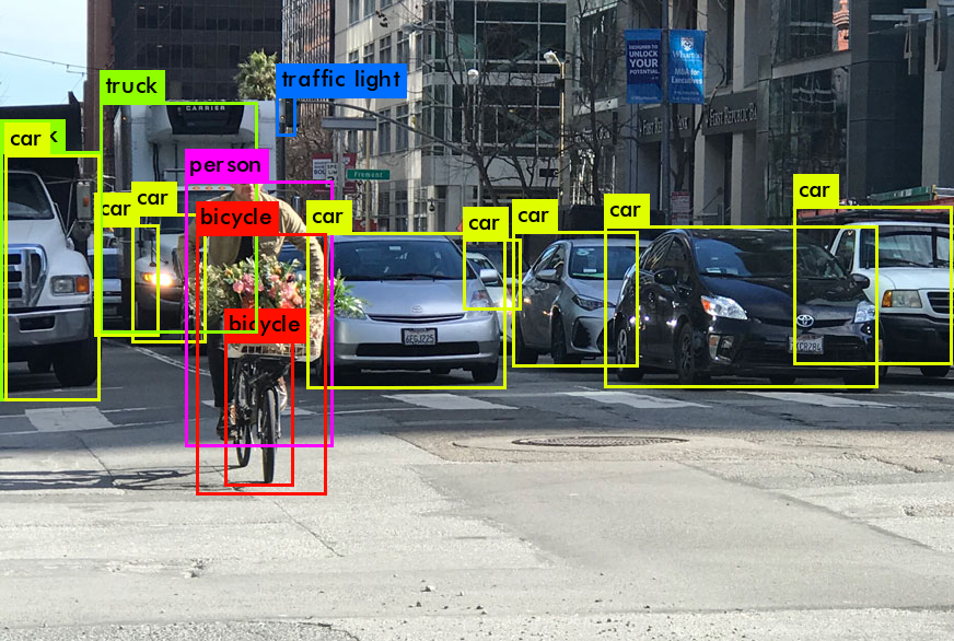
High-scoring regions are noted as positive detections of whatever class they most closely identify with. For example, while working on a live feed of traffic, YOLO can detect the different kinds of vehicles by "looking" into the regions where the score is high in comparison to predefined classes of vehicles.

3. A walkthrough of YOLOv3 architecture

This section goes through the change in architectures of previous versions of YOLO up to the point of YOLOv3.

3.1 YOLOv1 architecture

YOLOv1 was a 1-stage detector by using batch normalization (BN) and leaky ReLU activations, techniques that were relatively new at the time. Currently, YOLOv1 is pretty outdated and lacks some of the strong features that were introduced later.

3.2 YOLOv2 architecture

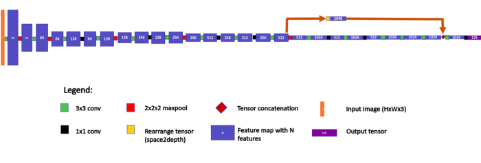
YOLOv2 contained a total of 22 convolutions and 5 maxpool operations. Feature map height represents spatial resolution. The above image is a 125-feature output for VOC PASCAL dataset with 20 classes and 5 anchors.

The authors of YOLOv1 completely removed the fully connected layer at the end while making YOLOv2. This opened up the gateway of the network to be resolution independent, meaning that the network can fit any image of any resolution. However, that doesn't mean that the network will perform well on any resolution. YOLOv2 employed the use of resolution augmentation during training.

This was also the time when various other flavors of the network were made that were smaller in size, faster in computation albeit less accurate, like Tiny YOLOv2. Tiny YOLOv2 was just a simple, long chain of convolutional and maxpooling layers and did not have the intricate bypass and rearranging operations like YOLOv2.

3.3 YOLOv3 architecture

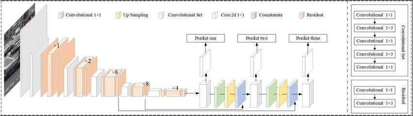
The architecture of YOLOv3 feature detector was inspired by other famous architectures like ResNet and FPN (Feature Pyramid Network). Darknet-53, the name of YOLOv3 feature detector, had 52 convolutions with skip connections like ResNet and a total of 3 prediction heads like FPN enabling YOLOv3 to process image at a different spatial compression.

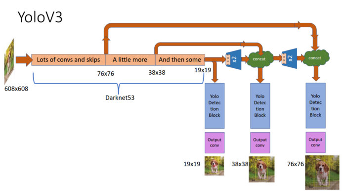
Like YOLOv2, YOLOv3 provides good performance over a wide range of input resolutions. Tested with input images of 608 x 608 in the COCO-2017 validation set, YOLOv3 achieved a mAP (mean average precision) of 37 making it 17 times faster than its competitor Faster-RCNN-ResNet50, a faster-RCNN architecture that uses ResNet-50 as its backbone. Other architectures like Mobilenet-SSD were similar in time taken by YOLOv3 to detect the images but they scored an mAP of 30.

3.3.1 Feature Pyramid Network (FPN): The secret sauce

Developed in 2017 by FAIR (Facebook Aritficial Intelligence Research), a feature pyramid is a topology in which a feature map gradually decreases in spatial dimension but increases again and is concatenated with previous feature maps with corressponding sizes. The different sized feature maps are then fed to a distinct detection head. YOLOv3 uses three detection heads.

3.3.2 Three scale detection

YOLO being a fully convolutional network, detects at three different scales. The output generated from those detections is passed through a 1 x 1 kernel at those three different places.

The size of the detection filter is 1 x 1 x (B x (4 + 1 + C)) where B represents the number of bounding boxes the filter can predict, number "4" is for the four bounding box attributes and number "1" for objectness predictions (object confidence). Lastly, C is the number of class predictions. YOLOv3 is trained on the COCO dataset so B = 3 and C = 80. Putting those values, we get a filter size of 1 x 1 x 255.

The detection takes place at the following layers:

First, at the 82nd layer. The 81st layer has a stride of 32. If the image has dimensions 416 x 416, we will obtain a feature map of 13 x 13. One detection by our 1 x 1 detection kernel yields a detection feature map of 13 x 13 x 255.

Second, at the 94th layer where we obtain a detection feature map of 26 x 26 x 255.

Third, at the 106th layer where we obtain a detection feature map of 52 x 52 x 255.

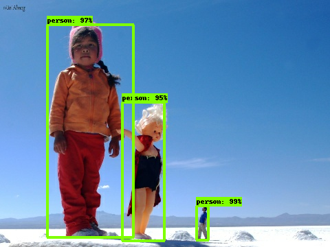
Now you might be wondering why three scales? Well, if we look at the image below, we can see the class "person" being detected three times for varying sizes. And that's your answer! YOLOv3 is capable of detecting at three different sizes because of those three detection feature maps. The first map of 16 x 16 is used for detection of large objects, 26 x 26 for medium objects and 52 x 52 for small objects. Furthermore, since the detection feature map for small object has a greater value, YOLOv3 is extremely accurate is detecting small objects.

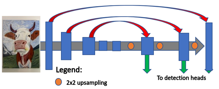
3.3.3 Upsampling and concatenation

The feature map is then taken from the previous two layers and upsampled by 2x. This portion covers the upsampling. Also, a feature map is taken from earlier part of the network and merged with the upsampled features. This covers the concatenation. This methodology is analogous to an encoder-decoder architecture.

By applying upsampling and concatenation, we are able to gather more semantic information and fine-grained informaation. A few more convolutional layers are added to process the encapsulated feature map, predicting a similar tensor with twice the size.

4. YOLOv3 high accuracy secret

YOLOv3 has a really small and simple topology, then how come it detects the images so easily and fast? Well, it all goes down to one thing. The more easy the structure, the difficult its math. Literally. The reason for such compact structure of YOLOv3 is because its loss function is really complicated. The loss gives the features its meaning. And the loss function of YOLOv3 is carefully crafted to encompass a lot of information into a small feature map.

4.1 Input resolution augmentation

YOLOv3 is a fully convolutional network as opposed to other networks having fully connected layers for classification. This enables the network to process images of any given size. But there is a problem. Such a network would give rise to a lot of network parameters. Thus, this problem is tackled by resolution augmentation.

The authors of YOLOv3 used 10 different resolution steps ranging from 384 x 384 to 672 x 672 pixels. Those resolutions alternate at random intervals every training batch which enables the network to generalize the predictions it made for different resolutions.

4.2 Loss coefficients: Divide and Conquer

In YOLOv3, each spatial cell in the output layer predicts multiple boxes. That number is 3 for YOLOv3. These boxes are centered in the cell and are called anchors.

The loss (YOLO loss) for every box prediction are based on the following terms.

1. Coordinate loss — if the prediction does not cover the object
2. Objectness loss — happens on an incorrect box-object IoU prediction
3. Classification loss — happens due to deviations from predicting ‘1’ for the correct classes and ‘0’ for all the other classes for the object in that box.

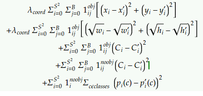
This is the loss function for YOLOv1. Looking at the second line, it used the width and height predictions (see the square root part). In YOLOv2 and YOLOv3, it was replaced by a residual scale prediction. This made the loss argument proportional to relative rather than absolute scale error.

5. What after YOLOv3?

In February 2020, the creator of YOLO, Joseph Redmond stopped his research in computer vision. But that didn't stop others to push a new update. Just two months after in April 2020, YOLOv4 came out which took inspiration from the state-of-the-art BoF (Bag of Freebies) and BoS (Bag of Specials) which increased the accuracy and inference cost respectively. This made YOLOv4 score 10% more in AP (average precision) and 12% in FPS (frames per second) than YOLOv3.

Another version of YOLO, YOLOv5 was released two months after YOLOv4. It was different from other releases as the previous releases were a fork from Darknet. YOLOv5 was a PyTorch implementation and had similarity with YOLOv4. Both had the CSP backbone and PA-NET neck. What made YOLOv5 different was the introduction of mosaic data augmentation and auto learning bounding box anchors.

This wraps up the overview of the YOLOv3 architecture. I hope you all liked this article at OpenGenus. Please read my other articles about algorithms and machine learning by viewing my profile.