
Get this book -> Problems on Array: For Interviews and Competitive Programming
In this article, we will be discussing Single Shot Detector (SSD), an object detection model that is widely used in our day to day life. And we will also see how the SSD works and what makes the SSD better than other object detection models out there.
Table of contents:
- Introduction to Single Shot Detector (SSD)
- What makes SSD special?
- Structure / Architecture of SSD model
- YOLO vs SSD
- Performance of SSD
- Conclusion
Let us get started with Single Shot Detector (SSD) + Architecture of SSD.
Introduction to Single Shot Detector (SSD)
SSD is an object detection model, but what exactly does object detection mean? A lot of people confuse object detection with image classification. In simple words, image classification says what the picture or image is, while object detection finds out the different things in the image and tells where they are in the image with the help of bounding boxes. With that cleared let's jump into SSD.
The famous single shot detectors are YOLO(you look only once) and Single Shot multibox detector. We will be discussing the SSD with a single-shot multibox detector since it is a more efficient and faster algorithm than the YOLO algorithm.
Single Shot detector the name of the model itself reveals most of the details about the model. Yes, the SSD model detects the object in a single pass over the input image, unlike other models which traverse the image more than once to get an output detection.
What makes SSD special?
As said above the SSD model detects objects in a single pass, which means it saves a lot of time. But at the same time, the SSD model also seems to have amazing accuracy in its detection.
In order to achieve high detection accuracy, the SSD model produces predictions at different scales from the feature maps of different scales and explicitly separates predictions by aspect ratio.
These techniques result in simple end-to-end training and high accuracy even on input images of low resolutions.
Structure / Architecture of SSD model
The SSD model is made up of 2 parts namely
- The backbone model
- The SSD head.
The Backbone model is a typical pre-trained image classification network that works as the feature map extractor. Here, the image final image classification layers of the model are removed to give us only the extracted feature maps.
SSD head is made up of a couple of convolutional layers stacked together and it is added to the top of the backbone model. This gives us the output as the bounding boxes over the objects. These convolutional layers detect the various objects in the image.
How does SSD work?
The SSD is based on the use of convolutional networks that produce multiple bounding boxes of various fixed sizes and scores the presence of the object class instance in those boxes, followed by a non-maximum suppression step to produce the final detections
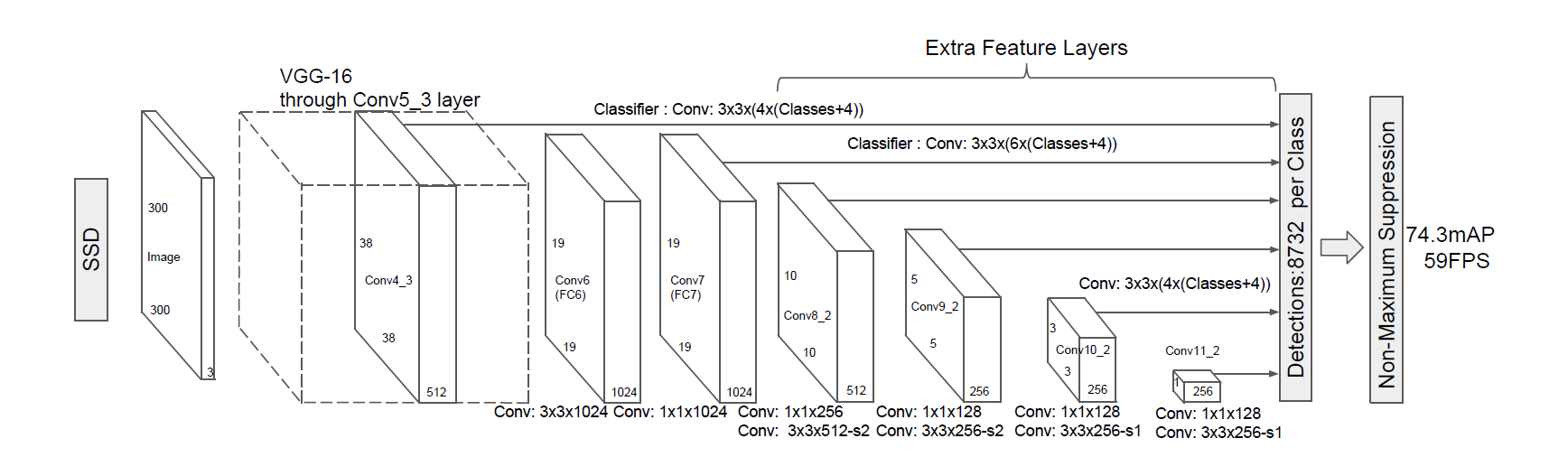
Note: In this model, we will be discussing the SSD built on the VGG-16 network as its backbone model. But the SSD can also be implemented using various other backbone models.
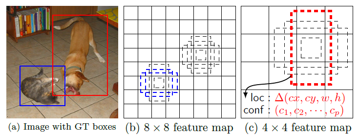
The SSD model works as follows, each input image is divided into grids of various sizes and at each grid, the detection is performed for different classes and different aspect ratios. And a score is assigned to each of these grids that says how well an object matches in that particular grid. And non maximum supression is applied to get the final detection from the set of overlapping detections. This is the basic idea behind the SSD model.
Here we use different grid sizes to detect objects of different sizes, for example, look at the image given below when we want to detect the cat smaller grids are used but when we want to detect a dog the grid size is increased which makes the SSD more efficient.
Let's dive into more details on how the objects are detected.
Detections using multi-scale feature maps
The multi-scale feature maps are added to the end of the truncated backbone model. These multi-scale feature maps reduce in size progressively, which allows the detections at various scales of the image. The convolutional layers used here vary for each feature layer.
Detection using the convolutional predictors
The addition of each extra layer produces a fixed number of predictions using the convolutional filters in them. These additional layers are shown at the top of the model in the given diagram below. For example, a feature layer of size m x n with p channels, the minimal prediction parameter that gives a decent detection is a 3 x 3 x p small kernel. Such kernel gives us the score for a category or a shape offset relative to the default box coordinates.
Usage of Default Boxes and aspect ratios
The default bounding boxes are associated with every feature map cell at the top of the network. These default boxes tile the feature map in a convolutional manner such that the position of each box relative to its corresponding cell is fixed.
For each box out of k at a given location, c class scores are computed and 4 offset relatives to the original default box shape. This results in the total of (c+4)k filters that are applied around each location in the feature map, yielding (c+4)kmn outputs for a feature map of size m x n.
This allows the usage of different default box shapes in several feature maps and makes the model efficiently discretize the space of possible output box shapes.
The table given below gives the details about all the operations in the SSD head
| Type / Name | Grid size | Kernel Size |
|---|---|---|
| Conv 6 | 19×19 | 3x3x1024 |
| Conv 7 | 19×19 | 1x1x1024 |
| Conv 8_2 | 10×10 | 1x1x256 3x3x512-s2 |
| Conv 9_2 | 5×5 | 1x1x128 3x3x256-s2 |
| Conv 10_2 | 3×3 | 1x1x128 3x3x256-s1 |
| Conv 11_2 | 1×1 | 1x1x128 3x3x256-s1 |
YOLO vs SSD
The You look only once (YOLO) model is a predecessor to the SSD model, it also detects images in a single pass, but it uses two fully connected layers while the SSD uses multiple convolutional layers. The SSD model adds several feature layers to the end of a base network, which predicts the offsets to default boxes of different scales and aspect ratios and their associated scores.
The SSD produces an average of 8732 detections per class while the YOLO produces only 98 predictions per class.
An SSD with a 300 x 300 inputs size significantly outperforms a 448 x 448 YOLO counterpart in accuracy as well as speed in the VOC2007 test.
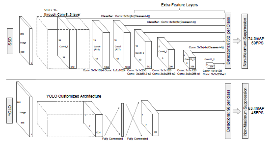
The image compares the SSD model with a YOLO model.
Performance of SSD
The SSD model is proven to show better results than the previous state-of-the-art detection algorithms like YOLO and Faster R-CNN. The multi-output layers at different resolutions have impacted the performance hugely, in fact, even removal of few layers resulted in a decrease in the accuracy by 12%.
| System | VOC2007 test mAP | FPS (Titan X) | Number of Boxes | Input resolution |
|---|---|---|---|---|
| Faster R-CNN (VGG16) | 73.2 | 7 | ~6000 | ~1000 X 600 |
| YOLO (customized) | 63.4 | 45 | 98 | 448 X 448 |
| SSD300* (VGG16) | 77.2 | 46 | 8732 | 300 X 300 |
| SSD512* (VGG16) | 79.8 | 19 | 24564 | 512 X 512 |
Performance comparison with other models
Conclusion
The SSD model is one of the fastest and efficient object detection models for multiple categories. And it has also opened new doors in the domain of object detection. With this article at OpenGenus, you must have the complete idea of SSD.
If you are interested to learn more about the Single shot multibox detector model feel free to check out the original research paper.