Connectionist models also known as Parallel Distributed Processing (PDP) models are used to model humans perception, cognition and behavior. They are used in different aspects like language processing, cognitive control, perception and memory. Neural Networks are by far the most used connectionist model and one of them is the Boltzmann Machine that we will cover in this article.

Table of Content

1. What is a Boltzmann Machine?
2. Generating data using a Boltzmann Machine
3. Training a Boltzmann Machine
4. Types of Boltzmann Machines
5. Applications of Boltzmann Machine
6. Limitations of Boltzmann Machine
7. Conclusion

1. What is a Boltzmann Machine?

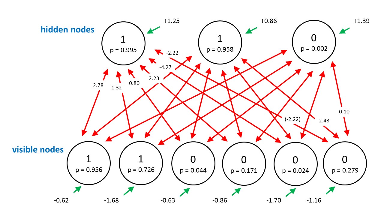
Boltzmann Machine (BM) is an unsupervised deep learning model used basically to discover features in datasets composed of binary vectors. The nodes in this network are symmetrically organized and each one is connected to every other node.
The connections between these nodes are undirected. Each connection (i,j) is associated with a weight wij. The weights are the parameters of the network. Large positive weights are indicators of high positive correlation between the nodes of the connection and large negative weights are indicators of high negative correlation.
Each node (i) is associated with a bias (bi). Also each node has a binary state (si) and makes a stochastic decision on whether to be ON or OFF.

Diagram of a Boltzmann Machine. Blue Nodes represent hidden nodes and whites nodes represent visible nodes.

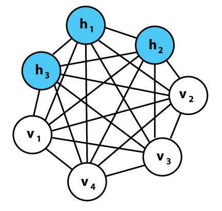
Boltzmann machines are composed of two types of nodes (as shown in the figure above):

1. Visible nodes: Have a visible state and they are responsible for receiving the binary input vectors and rendering the outputs (results).
2. Hidden nodes: Are probabilistic in nature, have a hidden state and they act like latent variables (features) that help the network model distributions over the visible nodes.

It is important to note that the visible nodes depend on the hidden nodes as much as the hidden nodes depend on the visible nodes, hence there is a circular dependency between the nodes.

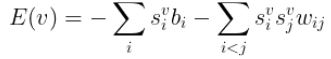
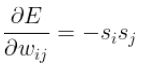
Boltzmann Machines are energy based models (EBM), because their objective function is an energy function, it is analogous to the loss function of a feed forward neural network. It is defined by the following equation :

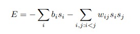
When the biases and the weights are highly positive then E<0, hence E is minimized, leading the nodes associated with those weights to have similar states (state attraction).
When the biases or the weights are highly negative then E > 0, leading the nodes associated with those weights to have different states (state repulsion).

Boltzmann machines are used to solve two different types of computational problems:

1. Search problems:In this case, the weights of the connections are fixed. They represent a cost function. The goal of the network is to generate (sample) binary state vectors that are solutions to the optimization problem. This is what makes BM a generative model.
2. Learning problems: Binary state vectors are fed to the network. The goal of the network in this case is to learn the weights that make the input a solution for the optimization problem represented by those weights.

2. Generating data using a Boltzmann Machine

A Boltzmann Machine generates data using an iterative process called Gibbs Sampling or Markov Chain Mont Carlo (MCMC) Sampling. This process works as follow:

• First the network is initialized with random states
• For each node, its conditional probability for being ON will be computed using the following equations

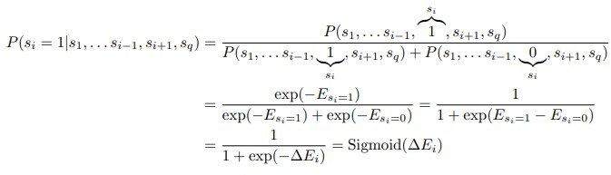
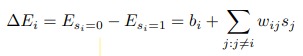
• Then the new states will be sampled using the previously calculated probabilities
• This process is repeated until the generated distribution becomes stationary.

Notes:

• When the generated distribution becomes stationary, we say that the network reached its thermal equilibrium.
• The time necessary to reach the thermal equilibrium is called the burn-in time

In equilibrium state, the generated data represents the model captured by the Boltzmann Machine. In this case, the probability of a state vector v will be dependent solely by the energy of this state vector relatively to all binary state vector. The probability used to generate data is calculated as follow:

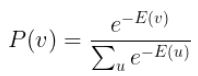
Where the energy of a state vector v is defined as :

3. Training a Boltzmann Machine

Training a BM consists of finding the weights and the biases that define a stationary distribution where the training vectors have high probability. This is equivalent to maximizing the log-likelihood of the specific training dataset. The log-likelihood of an individual state is computed by applying the logarithm function on the probability of that state vector in thermal equilibrium:

where :

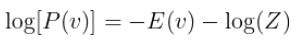
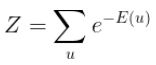
Z is called the partition function

Computing the derivative of the above function with respect to the weights wij requires computing the derivative of the energy function E and the derivative of the partition function Z.
knowing that :

It can be proved that:

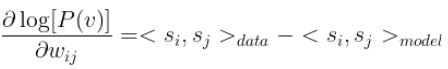
where:

• The first term represents data-centric samples. They are generated by fixing the visible states to a vector from the training dataset. Then running Gibbs sampling until reaching the thermal equilibrium. At that point, the hidden nodes provide the required samples and the visible nodes are clamped to the attribute of the corresponding data vector.
• The second term represents model-centric samples. They are generated by randomly initializing the visible and hidden states. Then running Gibbs sampling until the thermal equilibrium is reached.

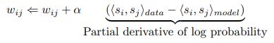
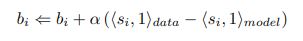
Once the above derivative is computed, the weights and biases will be updated using gradient ascent like follow:

4. Types of Boltzmann Machines

Restricted Boltzmann Machines

The standard Boltzmann Machine has a complex architecture that is hard to implement as the number of connections grows exponentially with the size of the network. To simplify the architecture, we apply a restriction on the connections between the nodes of the same type. This means that there will be no visible-visible connections or hidden-hidden connections. This type of architecture is called Restricted Boltzmann Machine (RBM).

Architecture of a Restricted Boltzmann Machine. [5]

The applied restriction comes with two advantages, first it simplifies the computation of the probabilities since the nodes of the same layer are now conditionally independent. Second the learning process is faster than in the standard architecture thanks to the reduced number of connections.

RBM can be trained just like standard BM, however, a more efficient algorithm exists and it is used to train them, it is called Contrastive Divergence Algorithm.

Conditional Boltzmann Machines

Boltzmann Machines are used to model distributions of data vectors. In order to do so they learn automatically the existing patterns in the given data which makes them more suitable for unsupervised learning tasks. However, they can also be used in supervised learning tasks where the goal is to predict the output that is conditioned on the input.
The equations will be the same, the only difference is in the learning process. When generating the model-centric samples, instead of randomly initializing the visible and the hidden nodes, a subset from the visible nodes will be clamped. The latter will act as the inputs and the remaining visible nodes will act as outputs.
Now the network will be maximizing the log probability of the observed output conditioned on the input vectors (the clamped visible nodes).

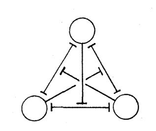
Higher-order Boltzmann Machines

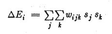
Boltzmann Machine is a non-linear network that models interactions between pairwise stochastic binary nodes. However, the learning algorithm of a BM can be extended to higher order interaction. This type of networks is used to faster the learning process. For example for order l=3 , we will have a weight wijk that is shared between three nodes as shown in the figure bellow

Third order interaction between three nodes [4].

Since a Boltzmann Machine is symmetric, we should have :

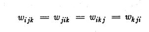
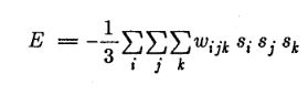
For simplicity reasons we will ignore the biases in the equations that follow.
The equation of the energy function E will become:

In Gibbs sampling, the conditional probability will be computed just like in standard BM, by applying the sigmoid function on the energy gap for node i. However the equation of the latter will be modified like the following :

Finally, the update rule will be the same except for the term sisj that will be replaced by sisjsk.

Boltzmann Machines with non-binary nodes

In standard Boltzmann Machines, the nodes have a binary state {0,1} and apply the sigmoid function to compute the probability of their state. However, in real life problems we may want to model a system with more than two states. In this case, the network can be generalized to use softmax units (nodes), Gaussian units, Poisson units or any unit using a probability function that falls in the exponential family which are characterized by the fact that the adjustable parameters have linear effects on the log probabilities.

5. Applications of Boltzmann Machines

Restricted Boltzmann Machines are the most successful type of Boltzmann Machines. They have been used in a wide range of applications.

5.1 Dimensionality reduction

The RBM's architecture is convenient for such type of problems since their hidden nodes are of lower dimension than their visible nodes, hence they have a reduced representation of the data.

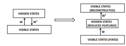
5.2 Data Reconstruction

RBM is an undirected graphical model. However, it can be shown to be equivalent to a directed graphical model with infinite number of layers.

Equivalence between undirected and directed RBM graph [2]

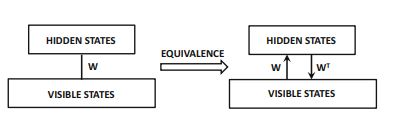
With this idea in mind, and with the idea that Auto-encoders (AE) are used to reconstruct data, we can unfold an RBM to approximate the AE architecture to perform the same task.

Using RBM to approximate auto-encoder [2]

5.3 Recommendation Engines

One of the most known applications for RBM is collaborative filtering where the network should provide a recommendation to the end user.
The basic idea behind recommender systems is to create a different training instance and a different RBM for each user, depending on the ratings provided by the users.
All RBMs share weights.
It is also important to notice that the ratings range from 1 to 5, hence we should use softmax nodes instead of sigmoid nodes, in order to correspond to the rating values.

Note:
The applications of Boltzmann Machines are not limited to the examples above, and they include also classification, regression, image restoration, object detection and also applications in signal processing. However, machine learning and deep learning practitioner have deprecated them in favor of more sophisticated models like Generative Adversarial Networks (GAN) and Variational Auto-encoders.

6. Limitations of Boltzmann Machines

Boltzmann machines suffer from many limitations that make them unsuitable for practical use.

• The learning process is very slow especially when the weights are large and the equilibrium distribution is multimodal.
• The generation of data using Boltzmann Machine is challenging compared to other generative models, because of the cyclic dependency between the nodes[2]
• Boltzmann Machine suffer from the variance-trap that causes the activations to saturate. This is harmful for the network because the nodes no longer outputs values between 0 and 1 [3] .

7. Conclusion

Boltzmann Machines are undirected generative models, composed of two types of nodes: visible nodes and hidden nodes. Each node is connected to all the other nodes. They have no output layer, both inputs and outputs are received on the visible nodes. Their goal is to learn the patterns and correlations inside the data. They can be used for both supervised and unsupervised learning tasks. Training them requires using Gibbs Sampling or Markov Chain Mont Carlo Sampling to reach the thermal equilibrium in which the generated distribution is stationary. They have been used in a wide range of applications: image processing, signal processing, classification, regression and dimensionality reduction. However due to their limitations they have been replaced by more sophisticated models.

References

[1] SOURIAU, Rémi, LERBET, Jean, CHEN, Hsin, et al. A review on generative Boltzmann networks applied to dynamic systems. Mechanical Systems and Signal Processing, 2021, vol. 147, p. 107072.

[2] AGGARWAL, Charu C. Artificial Intelligence-A Textbook. 2021

[3] Daniel L. Silver, et al. Dynamic Networks, March 2014. Available from: http://plato.acadiau.ca/courses/comp/dsilver/5013/Slides/Dynamic%20Networks.pptx

[4] SEJNOWSKI, Terrence J. Higher‐order Boltzmann machines. In : AIP Conference Proceedings. American Institute of Physics, 1986. p. 398-403.

[5] Build software better, together. GitHub [online]. [Accessed 17 October 2022]. Available from: https://github.com/topics/boltzmann-machines