
Get this book -> Problems on Array: For Interviews and Competitive Programming
Classification and Regression Trees (CART) is only a modern term for what are otherwise known as Decision Trees. Decision Trees have been around for a very long time and are important for predictive modelling in Machine Learning.
As the name suggests, these trees are used for classification and prediction problems. This is an introductionary post about the fundamentals of such decision trees, that serve the basis for other modern classifiers such as Random Forest.
These models are obtained by partitioning the data space and fitting a simple prediction model within each partition. This is done recursively. We can represent the partitioning graphically as a tree; hence the name.
They have withstood the test of time because of the following reasons:
- Very competitive with other methods
- High efficiency
Classification
Here our focus is to learn a target function that can be used to predict the values of a discrete class attribute, i.e. this is a classification problem where we want to know if, given labelled training data, something falls into one class or another. Naturally, this falls into Supervised Learning.
This includes applications such as approving loans (high-risk or low-risk), predicting the weather (sunny, rainy or cloudy).
Let us explore solving the classification problem using a decision tree example.
An Example Problem
Generally, a classification problem can be described as follows:
Data: A set of records (instances) that are described by:
* k attributes: A1, A2,...Ak
* A class: Discrete set of labels
Goal: To learn a classification model from the data that can be used to predict the classes of new (future, or test) instances.
Note- When our problem has 2 possible labels, this is called a Binary Classification Problem.
Eg - Predicting if someone's tumour is benign or malignant.
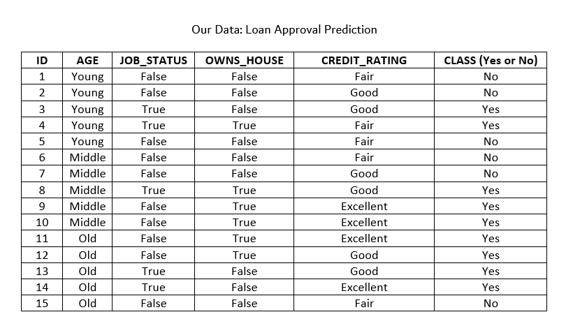
Our example problem is Loan Approval Prediction, and this is also a binary classification problem - either 'Yes' or 'No'. Each record is for one loan applicant at a famous bank. The attributes being considered are - age, job status, do they own a house or not, and their credit rating. In the real world, banks would look into many more attributes. They may even classify individuals on the basis of risk - high, medium and low.
Here is our data:
And here is the goal:
Use the model to classify future loan applications into one of these classes:
Yes (approved) and No (not approved)
Let us clasify the following applicant whose record looks like this:
Age: Young
Job_Status: False
Owns_House: False
Credit_Rating: Good
What would a decision tree look like for the above problem?
Here is one example of a decision tree -
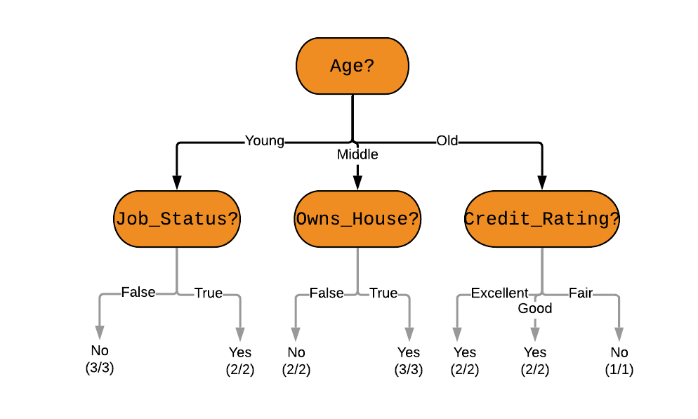
However, we must note that there can be many other possible decision trees for a given problem - we want the shortest one. We also want it to be better in terms of accuracy (prediction error measured in terms of misclassification cost).
Here is an alternative, shorter decision tree for the same -

All current tree building algorithms are heuristic algorithms. ID3 is an old algorithm that was invented by Ross Quinlan for creating effecient decision trees; in many ways a predecessor of the now popular C4.5 algorithm that he also created. Using such algorithms, we will be able to always arrive at a decision tree that works best. You can read more about them in the references below.
Another classic algorithm that was also invented around the same time as ID3 is called CART (not to be confused with the overall, modern term for decision trees). Let us try to create our own Decision Tree for the above problem using CART.
CART Algorithm for Classification
Here is the approach for most decision tree algorithms at their most simplest.
The tree will be constructed in a top-down approach as follows:
Step 1: Start at the root node with all training instances
Step 2: Select an attribute on the basis of splitting criteria (Gain Ratio or other impurity metrics, discussed below)
Step 3: Partition instances according to selected attribute recursively
Partitioning stops when:
There are no examples left
All examples for a given node belong to the same class
There are no remaining attributes for further partitioning – majority class is the leaf
What is Impurity?
The key to building a decision tree is in Step 2 above - selecting which attribute to branch off on. We want to choose the attribute that gives us the most information. This subject is called information theory.
In our dataset we can see that a loan is always approved when the applicant owns their own house. This is very informative (and certain) and is hence set as the root node of the alternative decision tree shown previously. Classifying a lot of future applicants will be easy.
Selecting the age attribute is not as informative - there is a degree of uncertainity (or impurity). The person's age does not seem to affect the final class as much.
Based on the above discussion:
- A subset of data is pure if all instances belong to the same class.
- Our objective is to reduce impurity or uncertainty in data as much as possible.
The metric (or heuristic) used in CART to measure impurity is the Gini Index and we select the attributes with lower Gini Indices first. Here is the algorithm:
//CART Algorithm
INPUT: Dataset D
1. Tree = {}
2. MinLoss = 0
3. for all Attribute k in D do:
    3.1. loss = GiniIndex(k, d)
    3.2. if loss<MinLoss then
        3.2.1. MinLoss = loss
        3.2.2. Tree' = {k}
4. Partition(Tree, Tree')
5. until all partitions procressed
6. return Tree
OUTPUT: Optimal Decision Tree
We need to first define the Gini Index, which is used to find the information gained by selecting an attribute. The Gini Index favours larger partitions and is calculated for i = 1 to the n, number of attributes:
Gini = 1 - ∑(pi)2
Here, pi is the probability that a tuple in D belongs to the class Ci.
Now, coming back to the example problem. We shall solve this in steps:
Step 1: Find Gini(D)
In our case, Gini(D) = 1 - (9/15)2 - (6/15)2 = 0.48
[since we have 9 Yes and 6 No class values for the 15 total records]
Step 2: Find Ginik(D) for each attribute k
Ginik(D) = ∑|Di|/|D| * Gini(Di)
For i = 1 to n, where Di is a partition of the dataset D
So, for the attribute Owns_House:
GiniOwns_House(D) = (5/15) * Gini(DOwns_House = True) + (10/15) * Gini(DOwns_House = False)
= (5/15) * [1 - (5/5)2 - (0/5)2] + (10/15) * [1 - (3/10)2 - (7/10)2]
= 0.28
And for the Age attribute:
GiniAge(D) = (5/15) * Gini(DAge = Young) + (5/15) * Gini(DAge = Middle) + (5/15) * Gini(DAge = Old)
= 0.33
Similarly, we can find the Gini Indices for the other attributes:
GiniCredit_Rating(D) = 0.634
GiniJob_Status(D) = 0.32
(try calculating these yourself!)
Step 3: Partition at Minimum Gini Index Values
As stated above, we need the root node of the decision tree to have the lowest possible Gini Index, and in our case that is the attribute Owns_House. The next attribute is Job_Status.
This is how we ultimately arrive at this decision tree -
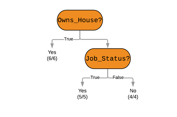
And using this decision tree for our problem - we can see that the applicant does not own a house, and does not have a job. Unfortunately, his loan will not be approved.
Prediction using CARTs
We saw that decision trees can be classified into two types:
Classification trees which are used to separate a dataset into different classes (generally used when we expect categorical classes). The other type are Regression Trees which are used when the class variable is continuous (or numerical).
Our focus is to learn a target function that can be used to predict the values of a continueous class attribute, i.e. this is a prediction problem where we want to know if, given labelled training data, something falls into one class or another. Naturally, this also falls into Supervised Learning.
Let us continue with the Loan Application approval problem, but add an attribute for each applicant - Salary. This is a continuous attribute ranging from zero (for applicants with no jobs), to near infinity. The age and credit rating attributes can also be represented with actual numerical values, instead of the categories they were before. Our new dataset can look like this:
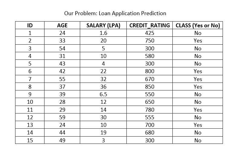
Now we can build a decision tree to predict loan approval on age, salary, credit rating, and various other variables. In this case, we are predicting values for the continuous variables. And the same CART algorithm we discussed above can be applied here. This is the biggest difference between CART and C4.5 (which will be introduced in a following post) - C4.5 cannot support numerical data and hence cannot be used for regression (prediction problems).
References
CARTs In Real World Applications - Image ClassificationTest Yourself
Question
Which of the following is NOT an algorithm for making decision trees?
With this article at OpenGenus, you must have the complete idea of Classification and Regression Trees (CART) Algorithm. Enjoy.