Dilated convolution, also known as Atrous Convolution or convolution with holes, first came into light by the paper "Semantic Image Segmentation with Deep Convolutional Nets and Fully Connected CRFs". The idea behind dilated convolution is to "inflate" the kernel which in turn skips some of the points. We can see the difference in the general formula and some visualization.

Table of content:

1. Introduction to Dilated Convolution
2. Dilated convolution in Tensorflow
3. Dilated convolution in action
4. Dilated Convolution: Results of the context module
5. Complexity analysis of dilated convolutions
6. Usefulness of Dilated Convolutions

We will dive into Dilated Convolution now.

Introduction to Dilated Convolution

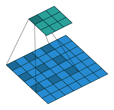
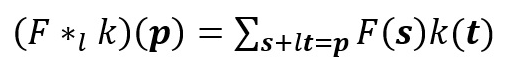
The following convolution represents the standard discrete convolution:

We see that the kernel looks up all the points of the input. The mathematical formula of discrete convolution is:

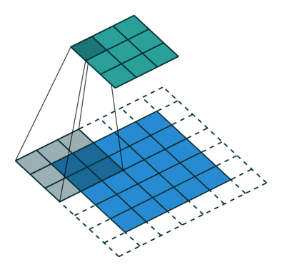
This represents dilated convolution:

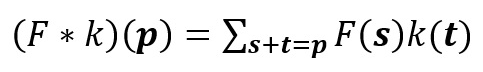
As you can clearly see, the kernel is skipping some of the points in our input. The mathematical formula of dilated convolution is:

We can see that the summation is different from discrete convolution. The l in the summation s+lt=p tells us that we will skip some points during convolution. When l = 1, we end up with normal discrete convolution. The convolution is a dilated convolution when l > 1. The parameter l is known as the dilation rate which tells us how much we want to widen the kernel. As we increase the value of l, there are l-1 gaps between the kernel elements. The following image shows us three different dilated convolutions where the value of l are 1, 2 and 3 respectively.

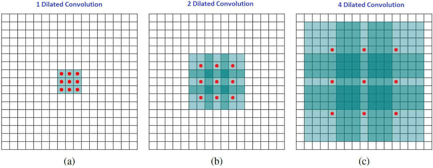
The red dots represent that the image we get after convolution is with 3 x 3 pixels. We see that the output of all three dilated convolutions have equal dimensions but the receptive field observed by the model is entirely different. Receptive field simply tells us how far the red dot can "see through". It is 3 x 3 when l=1, 5 x 5 when l=2, and 7 x 7 when l=3. The increase in receptive field means that we are able to observe more without any additional costs!

Dilated convolution in Tensorflow

Tensorflow has a built-in function for dilated convolution (or atrous convolution). The syntax for the dilated convolution function is:

tf.nn.atrous_conv2d(
    value, filters, rate, padding, name=None
)

This computes a 2-D atrous convolution, with a given 4-D value and filters tensors.

The rate parameters defines the dilation rate (l). If the rate parameter is equal to one, it performs regular 2-D convolution. If the rate parameter is greater than one, it performs atrous convolution, sampling the input values every rate pixels in the height and width dimensions.

Dilated convolution is similar if we are convolving the input with a set of upsampled filters, produced by inserting rate - 1 zeros between two consecutive values of the filters along the height and width dimensions.

The convolution is the most efficient when they are stacked on top of one another. A sequence of atrous_conv2d operations with identical rate parameters, 'SAME' padding, and filters with odd heights/widths:

    net = atrous_conv2d(net, filters1, rate, padding="SAME")
    net = atrous_conv2d(net, filters2, rate, padding="SAME")
    ...
    net = atrous_conv2d(net, filtersK, rate, padding="SAME")

can be equivalently performed cheaper in terms of computation and memory as:

    pad = ...  # padding so that the input dims are multiples of rate
    net = space_to_batch(net, paddings=pad, block_size=rate)
    net = conv2d(net, filters1, strides=[1, 1, 1, 1], padding="SAME")
    net = conv2d(net, filters2, strides=[1, 1, 1, 1], padding="SAME")
    ...
    net = conv2d(net, filtersK, strides=[1, 1, 1, 1], padding="SAME")
    net = batch_to_space(net, crops=pad, block_size=rate)

because each pair of consecutive space_to_batch and batch_to_space have the same block_size. Thus, they cancel each other out provided that their respective paddings and crops inputs are identical.

Dilated convolution in action

In the paper “Multi-scale context aggregation by dilated convolutions”, the authors build a network out of multiple layers of dilated convolutions. They increase the dilation rate l exponentially at each layer. As a result, while the number of parameters grows only linearly with layers, the effective receptive field grows exponentially with layers!

In the paper, a context module was made comprising of 7 layers that apply 3 x 3 convolutions with varying values of the dilation rate.

The dilation rates were 1, 1, 2, 4, 8, 16 and 1. The final convolution is a 1 x 1 convolution to make sure that the number of channels are the same as in the input one. This implies that the input and output has an equal number of channels.

At the bottom of the table, we can see two different types of output channels: Basic and Advanced. The Basic context module has only 1 channel (1C) in the whole module whereas the Advanced context module has increased the number of channels from 1C in the first layer to 32C at the penultimate layer (7th layer).

Dilated Convolution: Results of the context module

The model was tested on PASCAL VOC 2012 dataset. VGG-16 is used as the front-end module. Following was the setup of the model:

• The last two pooling and striding layers of VGG-16 were removed entirely, and the context module (discussed above) was plugged in.
• Padding of the intermediate feature maps was also removed.
• Padding of the input feature maps by a width of 33.
• A weight initialization considering the number of channels of input and output is used instead of standard random initialization.

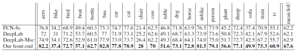
We can see that the dilated convolutions performed better than the previous FCN-8s and DeepLabV1 by about 5 percent on the test set. Also, a mean IoU (Intersection over Union) of 67.6% is also observed.

Complexity analysis of dilated convolutions

For any dilated convolution,

• There is a time complexity of O(d) for one dot product, which is simply d multiplications and d-1 addition.
• Since we perform k number of dot products, this amounts to O(k.d)
• Next, at the layer level, we apply our kernel n - k + 1 times over the input. If n >> k, this amounts to O(n.k.d)
• Finally, if we assume to have d number of kernels, our final time complexity of dilated convolution would be O(n.k.d^2).

Usefulness of Dilated Convolutions

Following are the advantages of using Dilated convolutions:

1. Since dilated convolutions support exponential expansion in the context of the receptive field, there is no loss of resolution.
2. Dilated convolutions use 'l' as the parameter for the dilation rate. As we increase the value of 'l' it allows one to have a larger receptive field which is really helpful as we are able to view more data points thus saving computation and memory costs.

While dilated convolutions provide a cheap way to increase the receptive field and helps in the saving computation costs, the main drawback of such methods
is the requirement for learning a large amount of extra parameters.

With this article at OpenGenus, you must have the complete idea of Dilated Convolution. Enjoy.

Read these Research papers:

• Semantic Image Segmentation with Deep Convolutional Nets and Fully Connected CRFs by Liang-Chieh Chen, George Papandreou, Iasonas Kokkinos, Kevin Murphy and Alan L. Yuille.
• Multi-Scale Context Aggregation by Dilated Convolutions by Fisher Yu and Vladlen Koltun