In this article, we will explore Empirical Risk Minimization (ERM) technique used in machine learning.

Table of contents

• What is risk?
• Empirical risk minimization
  
  

What is risk?

Before we get into empirical risk minimization, let us first get an understanding of what is risk.

In supervised learning, we use the dataset that is representative of all the classes for a given problem, to solve the problem. Let us consider an example of supervised learning problem - cancer diagnosis. Each input has a label 0 (cancer not diagnosed) or 1 (cancer diagnosed). Since we cannot have a data of all the people in the world, we sample out data of some people to be fed into our model. We use a loss function to find the difference between the actual diagnosis and the predicted diagnosis. This is essentially a measurement of error. In machine learning, 'risk' is synonymous to 'error'.

True risk is the average loss/error over all possibilities (here, the population of the whole world). Its formula is as follows:

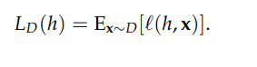
where h is the model and x is the data point.

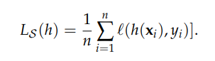
Since we use a small sample as the data for our model, we talk about empirical risk here. It is calculated as follows:

Computing true and empirical risk

Suppose we are working as a data analyst in a pharmaceutical company. For a particular drug under development, we need to compute if different samples of it yielded the required results based on its composition. First, we collect the dataset.

	Component 1	Component 2	y=yielded result?
Sample 1	0.8	0.8	0
Sample 2	0.3	0.25	1
Sample 3	0.2	0.8	1
Sample 4	0.3	0.7	1
Sample 5	0.9	0.7	0

Based on the above dataset, we develop a model h that takes in inputs of the percentage of both the components

x = (Component 1 (%),Component 2 (%)) and predicts y = 0 if Component 2 (%) > 0.5. Let us now compare our model's prediction with the actual ones.

	Component 1	Component 2	y=yielded result?	model prediction
Sample 1	0.8	0.8	0	0
Sample 2	0.3	0.25	1	1
Sample 3	0.2	0.8	1	0
Sample 4	0.3	0.7	1	0
Sample 5	0.9	0.7	0	0

To see how well our model has performed, we use the 0-1 loss function which simply charges 1 when the model is wrong and zero otherwise and compare the model's predictions with the actual ones. Then we compute the empirical risk as follows:

1\5 (0+0+1+1+0)= 2/5

For calculating the true risk, we need the entire distribution D that generates our dataset and also a true labeling function.

Let us assume that the amount of components 1 and 2 in D are selected in the interval [0,1] in a random, uniform and independent manner. Let the true labeling function be a function will label samples as h_T = 0 (did not yield result) if their c₁,c₂ combination is within distance 1/2 from the point [1,1]. The plot looks as follows:

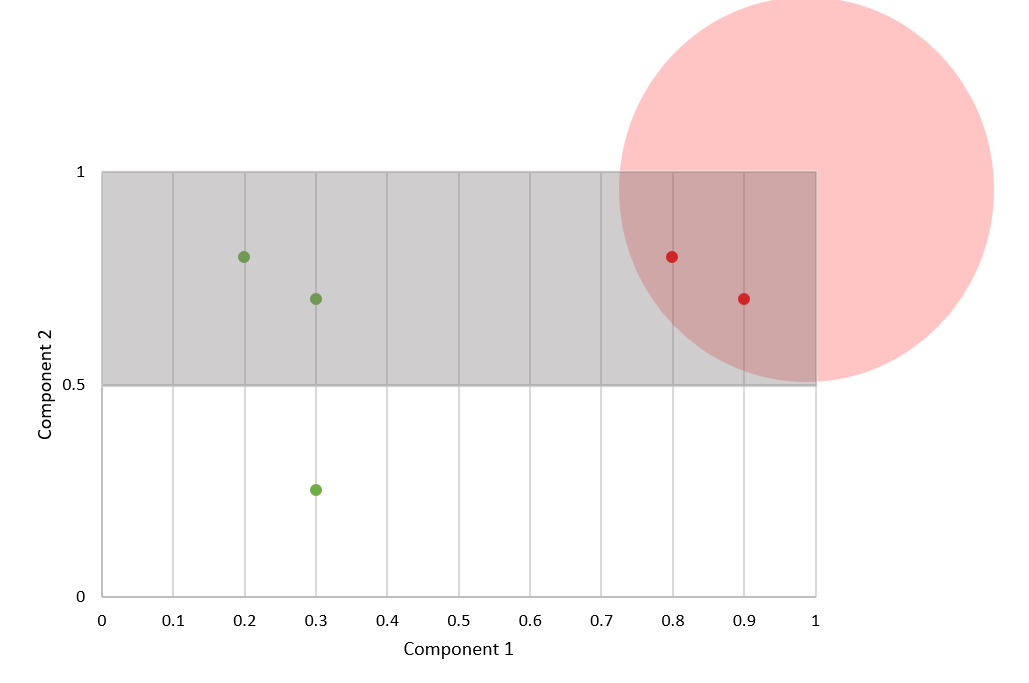
Here, the gray area is the condition where the model's prediction was 0 and the red circle represents the actual region where the sample did not yield results. Here, the difference between the area of the gray rectangle and the area of the quadrant gives the true risk.

True risk = 0.5 x 1 - 0.25 x 3.14 x (0.5)² = 0.30

Empirical Risk Minimization

While building our machine learning model, we choose a function that reduces the differences between the actual and the predicted output i.e. empirical risk. We aim to reduce/minimize the empirical risk as an attempt to minimize the true risk by hoping that the empirical risk is almost the same as the true risk.

Empirical risk minimization depends on four factors:

• The size of the dataset - the more data we get, the more the empirical risk approaches the true risk.
• The complexity of the true distribution - if the underlying distribution is too complex, we might need more data to get a good approximation of it.
• The class of functions we consider - the approximation error will be very high if the size of the function is too large.
• The loss function - It can cause trouble if the loss function gives very high loss in certain conditions.

The L2 Regularization is an example of empirical risk minimization.

L2 Regularization

In order to handle the problem of overfitting, we use the regularization techniques. A regression problem using L2 regularization is also known as ridge regression.

In ridge regression, the predictors that are insignificant are penalized. This method constricts the coefficients to deal with independent variables that are highly correlated. Ridge regression adds the “squared magnitude” of coefficient, which is the sum of squares of the weights of all features as the penalty term to the loss function.

Here, λ is the regularization parameter.

With this article at OpenGenus, you must have the complete idea of Empirical Risk Minimization.