In this article, we will explore manifold learning, which is extensively used in computer vision, data mining and natural language processing.

Table of contents

• Dimensionality
• Manifold learning
  
  

Dimensionality

Many datasets used in machine learning have a large number of features. Dimensionality refers to the number of attributes/features a dataset has. When the dimensions are high, calculations become difficult and makes training very slow. When we add more variables to a multivariate model, the more difficult it becomes to predict certain quantities. In high dimensional datasets, there is a lot of space between instances, making them sparse. This increases the chance of overfitting as the predictions will be based on much larger extrapolations. This is known as the curse of dimensionality. Statistically, it means that the more dimensions we add to the data, the sample size needed grows exponentially and quickly becomes difficult to manage.

Dimensionality reduction means reducing the dimensions of the data while maintaining its integrity. Manifold learning is an approach used for dimensionality reduction.

Manifold learning

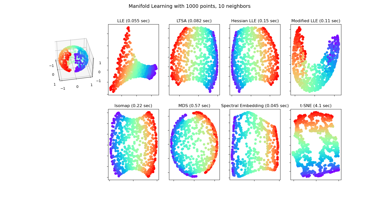
We can imagine 'manifold' to be a surface. It can be of any shape and not necessarily a plane. It can also contain curves. This is generalized to 'n' dimensions and is known as 'manifold' in mathematics. According to manifold hypothesis, the real world higher-dimensional data lie on lower-dimensional manifolds at most times. The process of modeling such manifolds where the data lies is called manifold learning. Given below is a visualization of different manifold learning methods.

These algorithms can be viewed as a non-linear version of Principal component analysis (PCA).

There are various approaches of manifold learning. They are:

• Isomap
• Multidimensional scaling (MDS)
• Locally Linear Embedding (LLE)
• Spectral embedding
• Modified Locally Linear Embedding (MLLE)
• Local Tangent Space Alignment
• t-distributed Stochastic Neighbor Embedding (t-SNE)
• Hessian Eigenmapping

Isomap

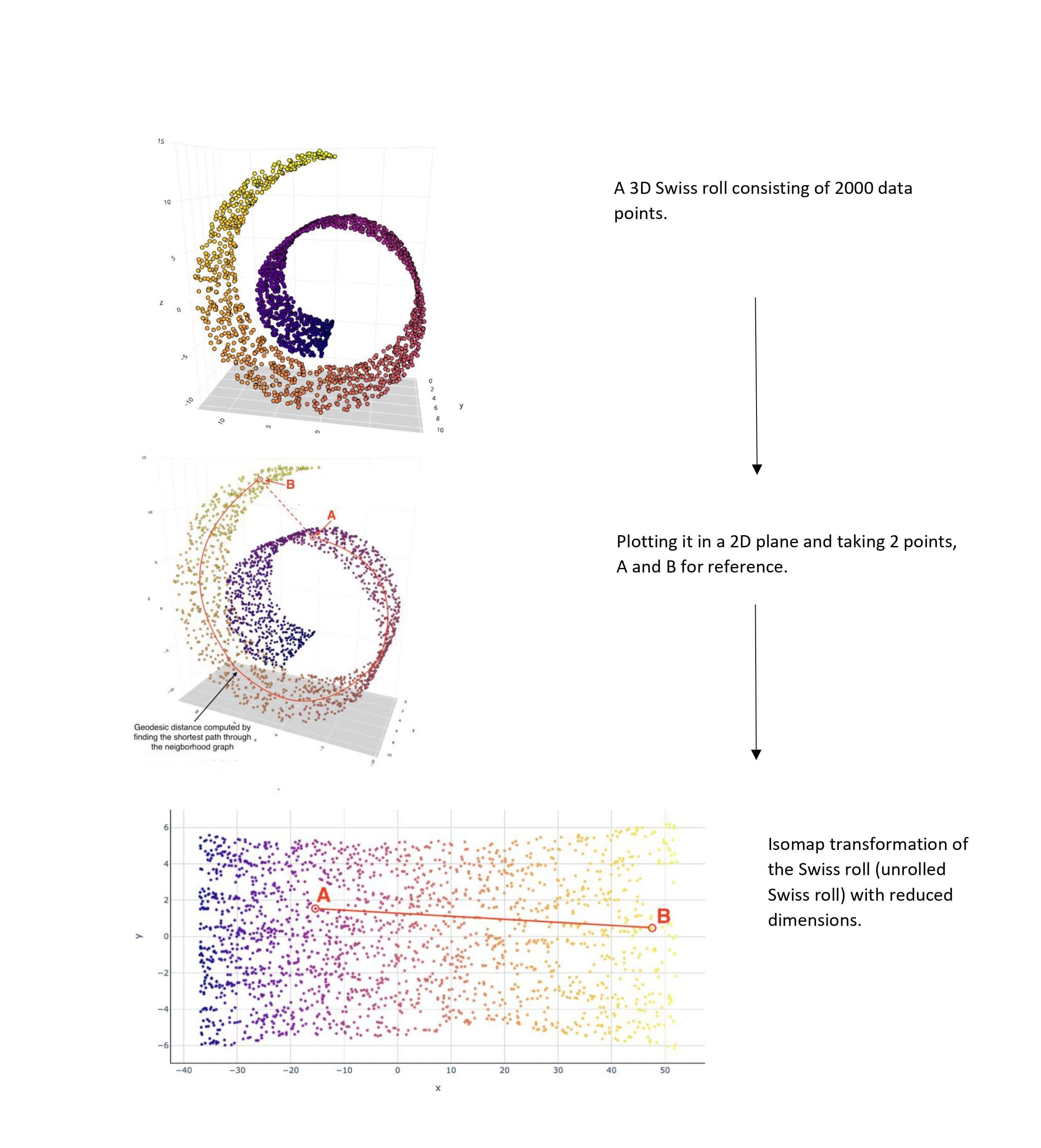
Isomap is the short form for Isometric Mapping. It is one of the earliest approach of manifold learning and is an unsupervised machine learning technique. It makes use of several different algorithms to reduce dimensions using a non-linear way. The steps performed by Isomap are:

1. Use KNN approach to find the k nearest neighbors.
2. After finding the neighbors, it maps the data points in a graph such that the points that are neighbors are connected and the points that are not neighbors remain unconnected. This is known as the neighborhood graph.
3. The shortest path between each pair of data points is found using algorithms like Dijkstra's or Floyd-Warshall algorithm.
4. Lower dimensional embedding is computed using multidimensional scaling.

Given below is an example of Isomap.

Multidimensional scaling (MDS)

Multidimensional scaling is a part of unsupervised learning algorithms for dimensionality reduction. It is of two types: metric MDS and non-metric MDS. Metric MDS is also known as Principle Coordinate Analysis (PCoA) and calculates the distances between data points to model the similarities or dissimilarities among them. It uses the geometric coordinates of the data points to calculate the distance between them. The two main steps this algorithm follows are:

1. Calculating distance between each pair of data points.
2. Finding a set of coordinates in lower-dimensional space that minimizes the stress. This is done as an attempt to solve the optimization problem.

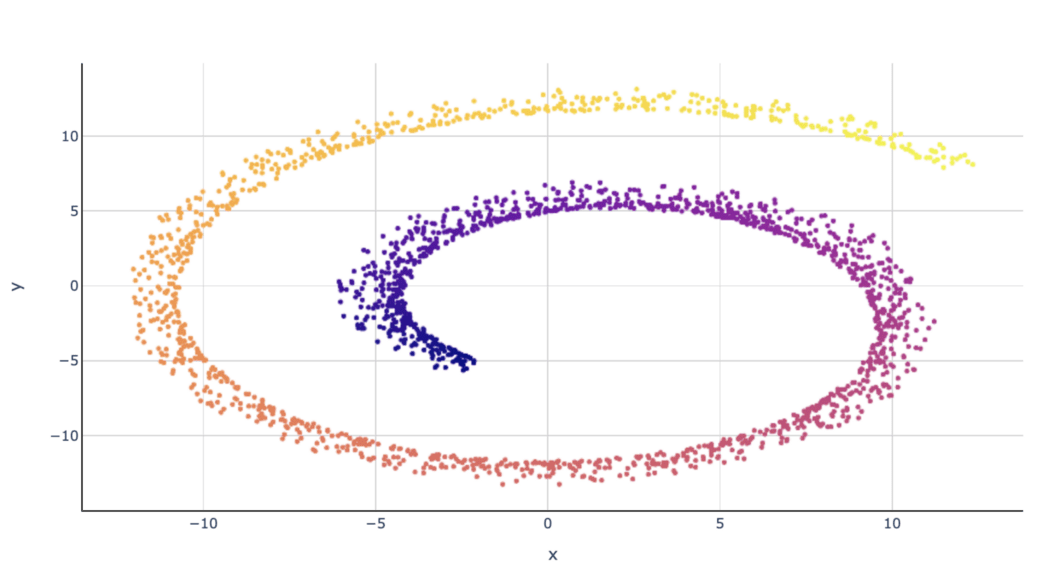
After MDS, the Swiss roll from our previous example looks as follows:

Locally Linear Embedding (LLE)

Locally Linear Embedding comes under unsupervised learning algorithms. Similar to isomap, LLE also combines several algorithms to reduce dimensions and give a lower level embedding. The steps followed in LLE are:

1. The KNN approach is used to find the k nearest neighbors.
2. A weight matrix is constructed. Here, the weight of every point is determined by minimizing the error of the cost function shown below. Since every point is a linear combination of its neighbors, the weights for non-neighbors are 0.
   
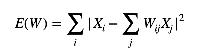
   Here, X_i is the position of the point of interest, X_j is the position of all the nearest neighbors and the sum of weights for each X_i is 1 i.e Σ_j W_ij=1.
3. The positions of all points in the lower-dimensional embedding are found by minimizing the cost function shown below. This provides us a lower dimensionality representation of our data.
   
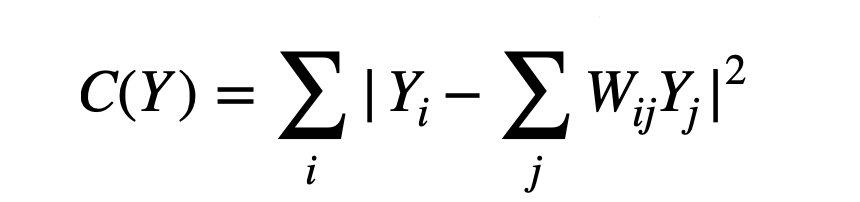
   Here, W is the weights from step 2.

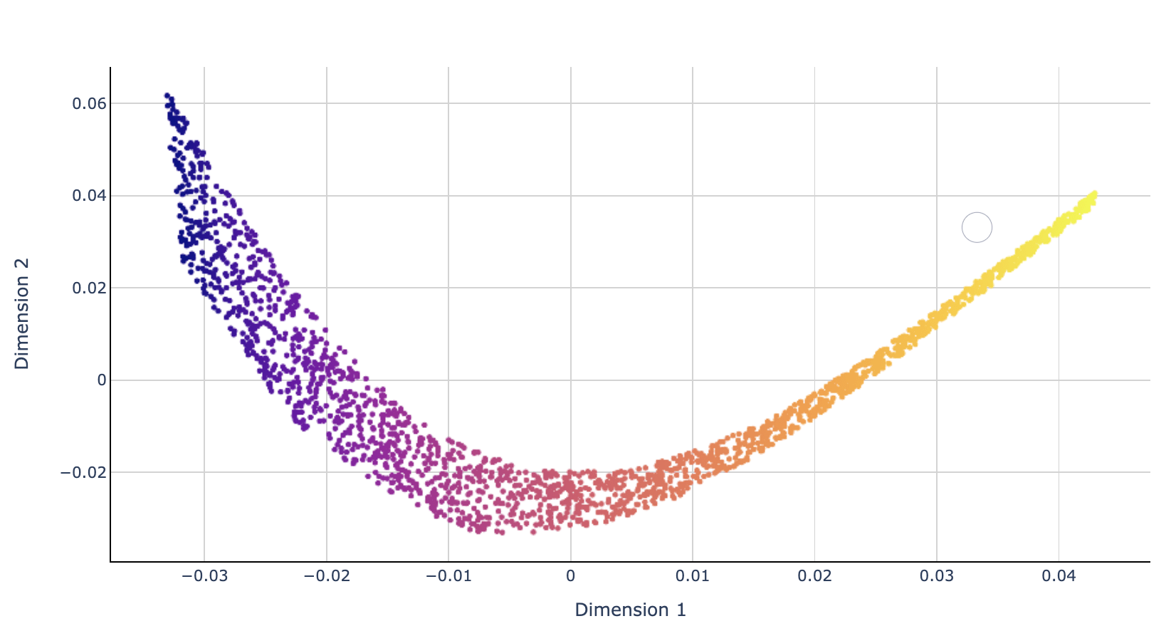
The result of LLE performed on the swiss roll is given below.

t-distributed Stochastic Neighbor Embedding (t-SNE)

This is another unsupervised learning algorithm used for visualizing high-dimensional data, gives us a feel of how data is organized in a higher dimensional space and also dimensionality reduction. It focuses on keeping similar data points close to each other in the low-dimensional space. The basic steps followed are:

1. Pairwise similarities between data points in the high-dimensional space are found. The Euclidean distances between data points in high-dimensional space are converted into probabilities and these conditional probabilities are then symmetrized to get the final similarities.
2. Each point in the higher dimensional space is mapped to a lower dimensional map based on the pairwise similarities calculated in the previous step. We use a Student t-distribution with one degree of freedom to model the points.
3. We want both the high and low dimensional map structures to be similar. Hence we find the difference between the probabilities in both the dimensions using KL divergence and then minimize the cost of our KL divergence using gradient descent.

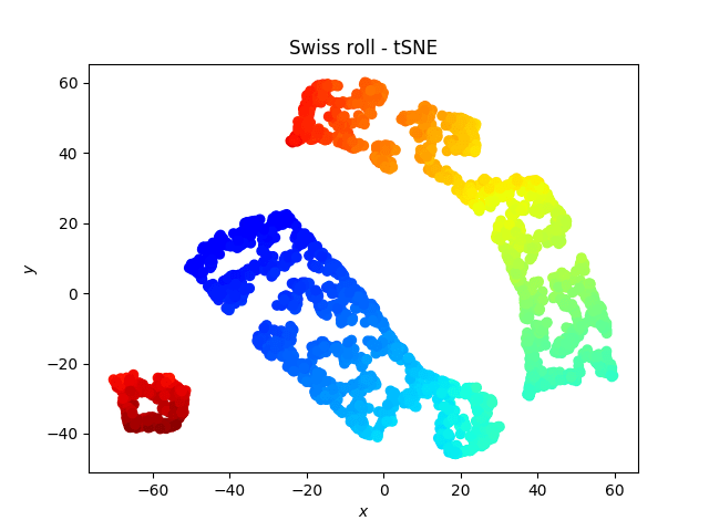
Swiss roll after t-SNE looks as follows:

Local Tangent Space Alignment

The Local Tangent Space Alignment (LTSA) can be considered as a variant of Locally-Linear Embedding (LLE). Instead of preserving the neighborhood distance like LLE, LTSA prioritizes characterizing the local geometry of each neighborhood. This builds up on the intuition that all the tangent hyperplanes will get aligned if a manifold is properly unfolded.

The first step here is same as LLE where the k-nearest neighbors are computed for every data point. Then first d principle components in each neighborhood is found and a weight matrix is constructed. Then similar to LLE, Partial Eigenvalue Decomposition is performed to find an embedding that aligns the tangent spaces.

With this article at OpenGenus, you must have the complete idea of Manifold Learning.