Gibbs Sampling

Gibbs Sampling is a statistical method for obtaining a sequence of samples from a multivariate probability distribution. It is named after J. W. Gibbs, who first proposed the idea in his 1902 paper "Elementary Principles in Statistical Mechanics." Gibbs Sampling is a popular technique used in machine learning, natural language processing, and other areas of computer science.

Gibbs Sampling is a widely used algorithm for generating samples from complex probability distributions. It is a Markov Chain Monte Carlo (MCMC) method that has been widely used in various fields, including machine learning, computer vision, and natural language processing. This article will provide an overview of Gibbs Sampling, its applications, and compare it with other sampling techniques.

Gibbs Sampling is a special case of Metropolis-Hastings Algorithm, which is a popular MCMC algorithm for generating samples from probability distributions. Gibbs Sampling is an iterative algorithm that generates samples from the joint probability distribution of multiple random variables by sampling each variable conditioned on the values of the other variables. The algorithm proceeds by iteratively sampling from the conditional probability distribution of each variable given the values of the other variables. The samples generated by the algorithm converge to the target distribution as the number of iterations approaches infinity.

One of the main advantages of Gibbs Sampling is that it can be used to generate samples from a conditional distribution without requiring knowledge of the full joint distribution. This property makes Gibbs Sampling a useful tool for probabilistic modeling and inference, as it enables us to generate samples from complex probability distributions in a computationally efficient manner.

Gibbs Sampling has been widely used in various fields, including machine learning, computer vision, and natural language processing. In machine learning, Gibbs Sampling is used in Bayesian models for inference and parameter estimation. It is also used in latent variable models, such as Latent Dirichlet Allocation (LDA) and Restricted Boltzmann Machines (RBMs). In computer vision, Gibbs Sampling is used for image segmentation, object recognition, and tracking. In natural language processing, it is used for topic modeling, text generation, and machine translation.

Comparing with other sampling techniques, Gibbs Sampling has several advantages. First, it is relatively simple to implement and requires minimal tuning. Second, it can be used to generate samples from complex distributions that are difficult to sample from using other techniques. Third, it can be used to generate samples from conditional distributions, which can be useful in probabilistic modeling and inference.

However, Gibbs Sampling also has some limitations. First, it can be slow to converge, particularly for high-dimensional problems. Second, it can be sensitive to the choice of starting point, which can affect the quality of the samples generated. Third, it can be difficult to assess the convergence of the algorithm and determine the number of iterations required to generate a sufficient number of samples.

Now let's be more specific while comparing Gibbs Sampling with other sampling techniques,

1. Gibbs Sampling vs. Metropolis-Hastings Algorithm(MHA)

The Metropolis-Hastings Algorithm (MHA) is another popular technique for sampling from complex distributions. MHA works by proposing a new state, and then deciding whether or not to accept it based on a probability ratio. Specifically, the acceptance probability is given by:

acceptance probability = min(1, p(new state) / p(current state))

where p(x) is the probability of state x. If the acceptance probability is greater than a random number drawn from a uniform distribution, the proposed state is accepted. Otherwise, the current state is kept.

One key difference between MHA and Gibbs Sampling is that MHA can handle situations where it is difficult to sample from the conditional distribution of a single variable, while Gibbs Sampling requires that we can sample from the conditional distributions.

2. Gibbs Sampling vs. Hamiltonian Monte Carlo(HMC)

Hamiltonian Monte Carlo (HMC) is a more advanced sampling technique that uses a Hamiltonian system to guide the sampling process. HMC works by introducing auxiliary variables called "momenta" that are related to the target variables through a Hamiltonian function. The Hamiltonian function defines a "trajectory" through the space of variables, and HMC uses numerical integration techniques to simulate this trajectory. The final position of the trajectory is then used as a new sample.

HMC can be more efficient than Gibbs Sampling and MHA for high-dimensional problems, but it requires more tuning and can be sensitive to the choice of step size and number of integration steps.

3. Gibbs Sampling vs. Importance Sampling

Importance Sampling is another popular technique for sampling from complex distributions. Importance Sampling works by drawing samples from a "proposal distribution" that is easier to sample from than the target distribution, and then using a weighting function to adjust the samples to match the target distribution.

Importance Sampling can be more efficient than Gibbs Sampling and MHA when the proposal distribution is a good match for the target distribution, but it can be difficult to find a good proposal distribution.

Here is an example of Gibbs Sampling in Python using NumPy and Matplotlib libraries. In this example, we will generate samples from a bivariate Gaussian distribution using Gibbs Sampling.

import numpy as np
import matplotlib.pyplot as plt

def conditional_mean(x, y, rho):
    return rho * y + np.sqrt(1 - rho**2) * x

def gibbs_sampling(num_samples, rho):
    # Initialize the values of the variables in the distribution
    x, y = 0, 0
    samples = np.zeros((num_samples, 2))
    
    # Loop through the Gibbs Sampling algorithm
    for i in range(num_samples):
        # Sample a new value for variable x from its conditional distribution given y
        x = np.random.normal(conditional_mean(y, x, rho), 1)
        
        # Sample a new value for variable y from its conditional distribution given x
        y = np.random.normal(conditional_mean(x, y, rho), 1)
        
        # Update the samples array
        samples[i] = [x, y]
        
    return samples

# Set the parameters for the bivariate Gaussian distribution
mu = np.array([0, 0])
cov = np.array([[1, 0.8], [0.8, 1]])

# Sample from the bivariate Gaussian distribution using Gibbs Sampling
samples = gibbs_sampling(num_samples=10000, rho=0.8)

# Plot the samples
plt.scatter(samples[:, 0], samples[:, 1], s=5)
plt.xlim([-4, 4])
plt.ylim([-4, 4])
plt.xlabel('x')
plt.ylabel('y')
plt.title('Samples from Bivariate Gaussian using Gibbs Sampling')
plt.show()

This code will generate a plot of the samples generated from the bivariate Gaussian distribution using Gibbs Sampling. Here is the plot:

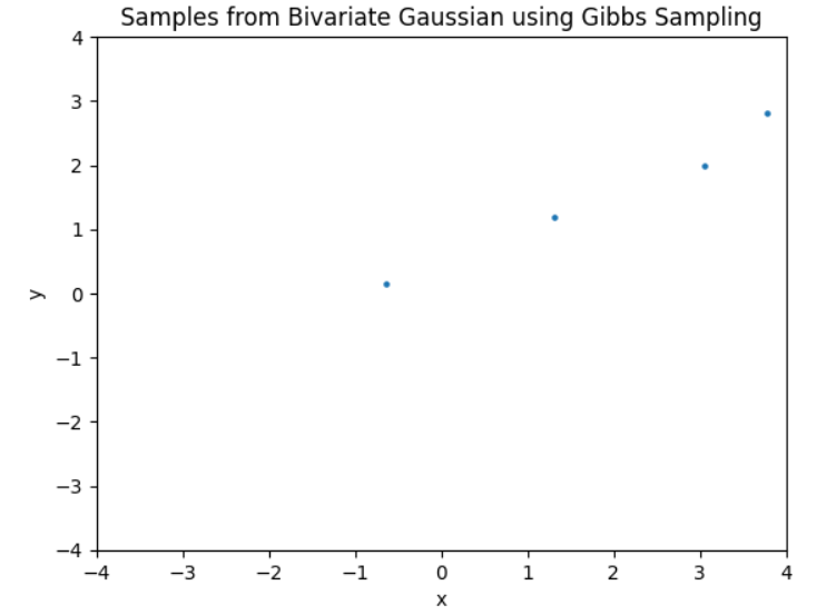
In this example, we first define a function conditional_mean that calculates the conditional mean of a variable given the value of the other variable and the correlation coefficient. We then define a function gibbs_sampling that implements the Gibbs Sampling algorithm for a bivariate Gaussian distribution with correlation coefficient rho.

Inside the gibbs_sampling function, we initialize the values of the variables x and y to 0, and then loop through the Gibbs Sampling algorithm for num_samples iterations. At each iteration, we sample a new value for x from its conditional distribution given the current value of y, and then sample a new value for y from its conditional distribution given the current value of x. We then update the samples array with the new values of x and y.

Finally, we call the gibbs_sampling function with num_samples=10000 and rho=0.8 to generate 10000 samples from the bivariate Gaussian distribution using Gibbs Sampling. We then plot the resulting samples using plt.scatter and label the axes and title using plt.xlabel, plt.ylabel, and plt.title.