Hopfield Network

Reading time: 30 minutes | Coding time: 10 minutes

Hopfield Network is a recurrent neural network with bipolar threshold neurons. In this article, we will go through in depth along with an implementation. Before going into Hopfield network, we will revise basic ideas like Neural network and perceptron.

A neural network is a mathematical model or computational model inspired by biological neural networks. It consists of an interconnected group of artificial neurons. The sructure and functioning of the central nervous system constituing neurons, axons, dentrites and syanpses which make up the processing parts of the biological neural networks were the original inspiration that led to the developement of computational models of neural networks.

The first computational model of a neuron was presented in 1943 by W. Mc Culloch and W. Pitts. They called this model threshold logic.The model paved the way for neural network research to split into two distinct approaches. One approach focused on biological processes in the brain and the other focused on the application of neural networks to artificial intelligence.

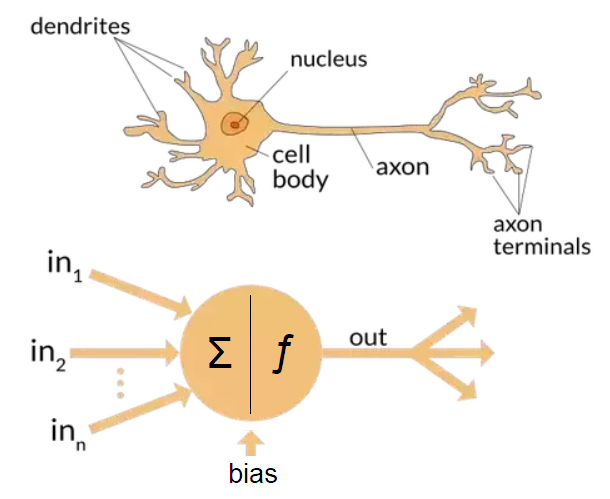
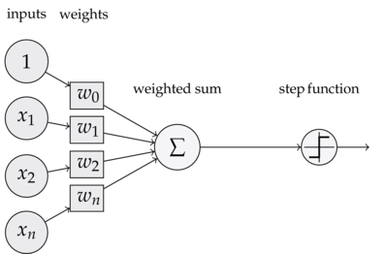
In 1958, Rossenblatt conceived the Perceptron, an algorithm for pattern recognition based on a two-layer learning computer network using simple addition and subtractio. His work had big repercussion but in 1969 a violent critic by Minsky and Papert was published.

The work on neural network was slow down but John Hopfield convinced of the power of neural network came out with his model in 1982 and boost research in this field. Hopfield Network is a particular case of Neural Network. It is based on physics, inspired by spin system.

The Network

Hopfield Network is a recurrent neural network with bipolar threshold neurons. Hopfield network consists of a set of interconnected neurons which update their activation values asynchronously. The activation values are binary, usually {-1,1}. The update of a unit depends on the other units of the network and on itself.

A neuron in Hopfield model is binary and defined by the standard McCulloch-Pitts model of a neuron:

where n_i(t+1) is the i^th neuron at time t+1, n_j(t) is the j^th neuron at time t, w_ij is the weight matrix called synaptic weights , θ is the step function and μ is the bias.In the Hopfield model the neurons have a binary output taking values -1 and 1. Thus the model has following form:

where S_i and n_i are related through the formula: S_i = 2n_i - 1 (Since n_i ϵ [0,1] and S_i ϵ [-1,1] ). ϑ_i is the thresold, so if the input is above the threshold it will fire 1. So here S represents the neurons which were represented as n in equation 1. The sgn sign here is the signum function which is described as follow:

For ease of analysis in this post we will drop the threshold (ϑ_i = 0) as we will analyse mainly random patterns and thresholds are not useful in this context. In this case the model is written as:

Training the Network

In this post we are looking at Autoassociative model of Hopfield Network. It can store useful information in memory and later it is able to reproduce this information from partially broken patterns.

For training procedure, it doesn’t require any iterations. It includes just an outer product between input vector and transposed input vector to fill the weighted matrix w_ij (or synaptic weights) and in case of many patterns it is as follow:

The main advantage of Autoassociative network is that it is able to recover pattern from the memory using just a partial information about the pattern. There are two main approaches to this situation.
We update the nuerons as specified in equation 3:

• Syncronously: Update all the neurons simultaneously at each time step;
• Asyncronously: At each time step, select at random, a unit i and update it.

Implementation

Now that we have covered the basics lets start implementing Hopfield network.

import matplotlib.pyplot as plt
import numpy as np

nb_patterns = 4   # Number of patterns to learn
pattern_width = 5
pattern_height = 5
max_iterations = 10

# Define Patterns
patterns = np.array([
   [1,-1,-1,-1,1,1,-1,1,1,-1,1,-1,1,1,-1,1,-1,1,1,-1,1,-1,-1,-1,1.],   # Letter D
   [-1,-1,-1,-1,-1,1,1,1,-1,1,1,1,1,-1,1,-1,1,1,-1,1,-1,-1,-1,1,1.],    # Letter J
   [1,-1,-1,-1,-1,-1,1,1,1,1,-1,1,1,1,1,-1,1,1,1,1,1,-1,-1,-1,-1.],     # Letter C
   [-1,1,1,1,-1,-1,-1,1,-1,-1,-1,1,-1,1,-1,-1,1,1,1,-1,-1,1,1,1,-1.],], # Letter M 
   dtype=np.float)

So we import the necessary libraries and define the patterns we want the network to learn. Here, we are defining 4 patterns. We can visualise them with the help of the code below:

# Show the patterns
fig, ax = plt.subplots(1, nb_patterns, figsize=(15, 10))

for i in range(nb_patterns):
    ax[i].matshow(patterns[i].reshape((pattern_height, pattern_width)), cmap='gray')
    ax[i].set_xticks([])
    ax[i].set_yticks([])

Which gives the out put as :

We now train the network by filling the weight matrix as defined in the equation 4

# Train the network
W = np.zeros((pattern_width * pattern_height, pattern_width * pattern_height))

for i in range(pattern_width * pattern_height):
    for j in range(pattern_width * pattern_height):
        if i == j or W[i, j] != 0.0:
            continue
            
        w = 0.0
        
        for n in range(nb_patterns):
            w += patterns[n, i] * patterns[n, j]
            
        W[i, j] = w / patterns.shape[0]  
        W[j, i] = W[i, j]  

Now that we have trained the network. We will create a corrupted pattern to test on this network.

# Test the Network
# Create a corrupted pattern S
S = np.array(    [1,-1,-1,-1,-1,1,1,1,1,1,-1,1,1,1,1,-1,1,1,1,1,1,1,-1,-1,-1.],     
   dtype=np.float)
   
# Show the corrupted pattern
fig, ax = plt.subplots()
ax.matshow(S.reshape((pattern_height, pattern_width)), cmap='gray')

The corrupted pattern we take here simply edditing some bits in the pattern array of letter C. We can see the corrupted pattern as follow:

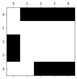
We pass the corrupted pattern through the network and it is updated as defined in the equation 3. Thus, after each iteration some update is applied to the corrupted matrix. We take the hamming distance of the corrupted pattern which is being updated every time and all the patterns. And then we decide the closest pattern in terms of least hamming distance.

h = np.zeros((pattern_width * pattern_height))
#Defining Hamming Distance matrix for seeing convergence 
hamming_distance = np.zeros((max_iterations,nb_patterns))
for iteration in range(max_iterations):
    for i in range(pattern_width * pattern_height):
        i = np.random.randint(pattern_width * pattern_height)
        h[i] = 0
        for j in range(pattern_width * pattern_height):
            h[i] += W[i, j]*S[j]
        S = np.where(h<0, -1, 1)
    for i in range(nb_patterns):
        hamming_distance[iteration, i] = ((patterns - S)[i]!=0).sum()   
    
    fig, ax = plt.subplots()
    ax.matshow(S.reshape((pattern_height, pattern_width)), cmap='gray')
hamming_distance

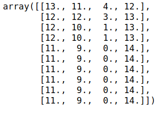
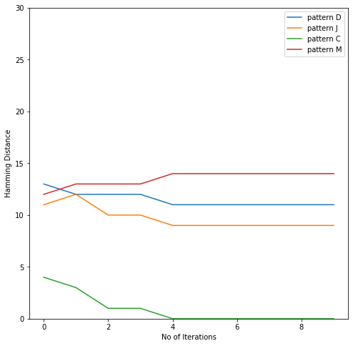
Here we see that the hamming distance between corrupted pattern and third pattern i.e. letter C has become 0 after few iterations thus correcting the corrupted pattern.

We can also see the plot for all the hamming distances below: