In this article, we will learn about what is Inception V3 model Architecture and its working. How it is better than its previous versions like the Inception V1 model and other Models like Resnet. What are its advantages and disadvantages?

Table of contents:

1. Introduction to Inception models
2. Inception V3 Model Architecture
3. Performance of Inception V3

Let us explore Inception V3 Model Architecture.

Introduction to Inception models

The Inception V3 is a deep learning model based on Convolutional Neural Networks, which is used for image classification. The inception V3 is a superior version of the basic model Inception V1 which was introduced as GoogLeNet in 2014. As the name suggests it was developed by a team at Google.

Inception V1

When multiple deep layers of convolutions were used in a model it resulted in the overfitting of the data. To avoid this from happening the inception V1 model uses the idea of using multiple filters of different sizes on the same level. Thus in the inception models instead of having deep layers, we have parallel layers thus making our model wider rather than making it deeper.

The Inception model is made up of multiple Inception modules.

The basic module of the Inception V1 model is made up of four parallel layers.

1. 1×1 convolution
2. 3×3 convolution
3. 5×5 convolution
4. 3×3 max pooling

Convolution - The process of transforming an image by applying a kernel over each pixel and its local neighbors across the entire image.

Pooling - Pooling is the process used to reduce the dimensions of the feature map. There are different types of pooling but the most common ones are max pooling and average pooling.

Here, different sizes of convolutions are performed to capture different sizes of information in the Picture.

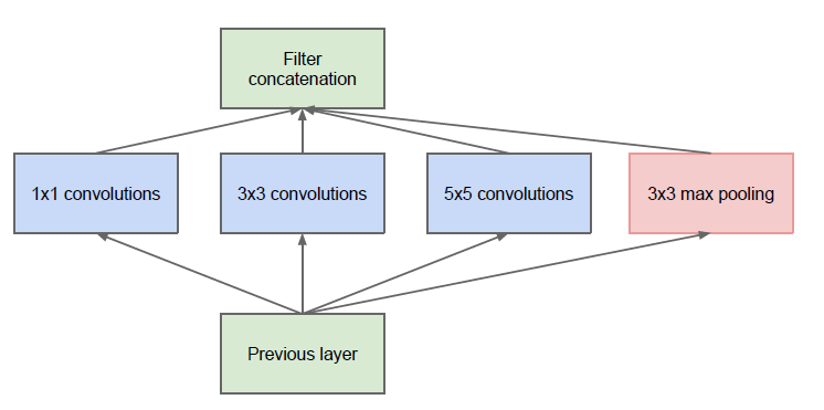
Naive Form

This module of the Inception V1 is called the Naive form. One of the drawbacks of this naive form is that even the 5×5 convolutional layer is computationally pretty expensive i.e. time-consuming and requires high computational power.

To overcome this the authors added a 1×1 convolutional layer before each convolutional layer, which results in reduced dimensions of the network and faster computations.

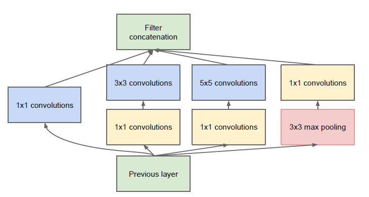
After adding the dimension reductions the module looks like this.

This is the building block of the Inception V1 model Architecture. The Inception V1 architecture model was better than most other models at that time. We can see that it has a very minimum error percentage.

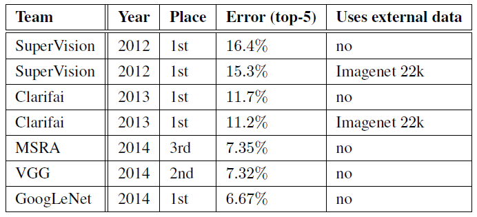
Comparison of Inception V1 with other models.

What makes the Inception V3 model better?

The inception V3 is just the advanced and optimized version of the inception V1 model. The Inception V3 model used several techniques for optimizing the network for better model adaptation.

• It has higher efficiency
• It has a deeper network compared to the Inception V1 and V2 models, but its speed isn't compromised.
• It is computationally less expensive.
• It uses auxiliary Classifiers as regularizes.

Inception V3 Model Architecture

The inception v3 model was released in the year 2015, it has a total of 42 layers and a lower error rate than its predecessors. Let's look at what are the different optimizations that make the inception V3 model better.

The major modifications done on the Inception V3 model are

1. Factorization into Smaller Convolutions
2. Spatial Factorization into Asymmetric Convolutions
3. Utility of Auxiliary Classifiers
4. Efficient Grid Size Reduction

Let's how each one of these optimizations was implemented and how it improved the model.

Factorization into Smaller Convolutions

One of the major assets of the Inception V1 model was the generous dimension reduction. To make it even better, the larger Convolutions in the model were factorized into smaller Convolutions.

For example, consider the basic module of the inception V1 module.

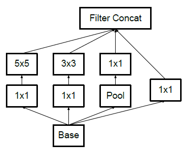
It has a 5×5 convolutional layer which was computationally expensive as said before. So to reduce the computational cost the 5×5 convolutional layer was replaced by two 3×3 convolutional layers as shown below.

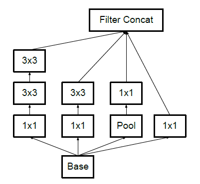
Module 2

To understand it better see how the process of using two 3×3 convolutions reduces the number of parameters.

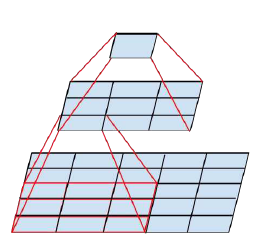
As a result of the reduced number of parameters the computational costs also reduce. This factorization of larger convolutions into smaller convolutions resulted in a relative gain of 28%.

Spatial Factorization into Asymmetric Convolutions

Even though the larger convolutions are factorized into smaller convolutions. You may wonder what if we can factorize furthermore for example to a 2×2 convolution. But, a better alternative to make the model more efficient was Asymmetric convolutions.

Asymmetric convolutions are of the form n×1.

So, what they did is replace the 3×3 convolutions with a 1×3 convolution followed by a 3×1 convolution. Doing so is the same as sliding a two-layer network with the same receptive field as in a 3×3 convolution.

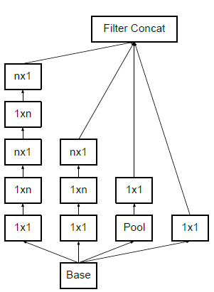
Module 2
Structure of Asymmetric Convolutions

The two-layer solution is 33% cheaper for the same number of output filters if the number of input and output filters is equal.

After applying the first two optimization techniques the inception module looks like this.

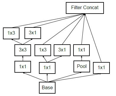
Module 3

Utility of Auxiliary classifiers

The objective of using an Auxiliary classifier is to improve the convergence of very deep neural networks. The auxiliary classifier is mainly used to combat the vanishing gradient problem in very deep networks.

The auxiliary classifiers didn't result in any improvement in the early stages of the training. But towards the end, the network with auxiliary classifiers showed higher accuracy compared to the network without auxiliary classifiers.

Thus the auxiliary classifiers act as a regularizer in Inception V3 model architecture.

Efficient Grid Size Reduction

Traditionally max pooling and average pooling were used to reduce the grid size of the feature maps. In the inception V3 model, in order to reduce the grid size efficiently the activation dimension of the network filters is expanded.

For example, if we have a d×d grid with k filters after reduction it results in a d/2 × d/2 grid with 2k filters.

And this is done using two parallel blocks of convolution and pooling later concatenated.

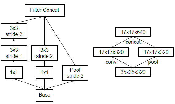
The above image shows how the grid size is reduced efficiently while expanding the filter banks.

The final Inception V3 model

After performing all the optimizations the final Inception V3 model looks like this

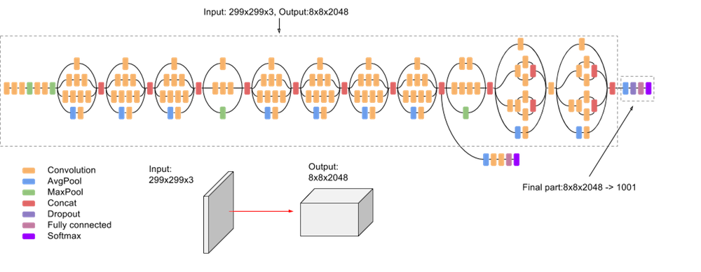
In total, the inception V3 model is made up of 42 layers which is a bit higher than the previous inception V1 and V2 models. But the efficiency of this model is really impressive. We will get to it in a bit, but before it let's just see in detail what are the components the Inception V3 model is made of.

Type	Patch / stride size	Input Size
Conv	3×3/2	299×299×3
Conv	3×3/1	149×149×32
Conv padded	3×3/1	147×147×32
Pool	3×3/2	147×147×64
Conv	3×3/1	73×73×64
Conv	3×3/2	71×71×80
Conv	3×3/1	35×35×192
3 × Inception	Module 1	35×35×288
5 × Inception	Module 2	17×17×768
2 × Inception	Module 3	8×8×1280
Pool	8 × 8	8 × 8 × 2048
Linear	Logits	1 × 1 × 2048
Softmax	Classifier	1 × 1 × 1000

The above table describes the outline of the inception V3 model. Here, the output size of each module is the input size of the next module.

Performance of Inception V3

As expected the inception V3 had better accuracy and less computational cost compared to the previous Inception version.

Multi-crop reported results.

We can see that the inception V3 model has an extremely low error rate compared with its previous models and its contemporaries.

Here are a few links if you are willing to know more details about the models

• Research paper of Inception V1 model
• Research paper of Inception V3 model

With this article at OpenGenus, you must have a complete idea of Inception V3 Model Architecture.