Least Absolute Deviation using ADMM

Least Absolute Deviation (LAD) is a powerful approach for solving optimization problems with good tolerance to outliers. Hence solving it to obtain a practicably applicable form is essential to take advantage of its theoretical prowess. For a better understanding, it is advised to have a good grasp of ADMM.

Table of contents

1. Introduction
2. Machine Learning Context
3. Solving the LAD Problem using ADMM
4. Implementation

Introduction

The names "least absolute deviation" (LAD), "least absolute errors" (LAE), "least absolute residuals" (LAR), and "least absolute values" (LAV) all refer to the same basic methodology. In 1757, Roger Joseph Boscovich established the idea of LAD, about 50 years before other absolute difference-based methods like Least Square (LS). Consideration of "Absolute values" offers a straightforward answer to the problem of comparing the predicted values to reality.

More specifically, LAD is a statistical optimality criterion and a technique for statistical optimization based on minimizing the sum of absolute deviations (also known as the sum of absolute residuals or sum of absolute mistakes) or the L1 norm of such values.

Machine Learning Context

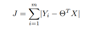
In Machine Learning, one of the main alternatives to the least-squares(∥Ax−b∥2^2) approach when attempting to estimate the parameters of regression is the LAD(∥Ax − b1∥1) method. The use of the absolute value results in a more robust solution for handling outliers and has the possibility of multiple solutions. The LAD cost is formulated as,

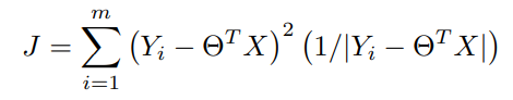
Now by Using the Weighted Least Square method we can write the same function as,

On rearranging the terms to obtain Θnew,

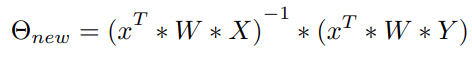
this serves as the update for Θ

Comparing L1 norm to L2 norm over a large range of values

Consider the plot of Loss vs Error of both the Norms,

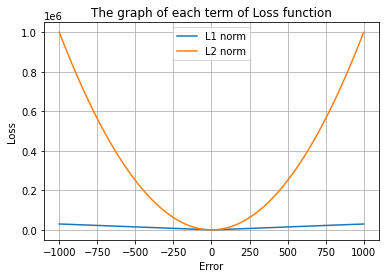
The hypothesis of handling outliers contained in data by penalizing the model less than the L2 norm will is supported by the plot, which shows that the L1 norm loss is much smaller than the L2 norm loss over a wide range of error values. As a result, there is no longer a requirement to strictly pre-process the data. So it makes sense to analyze this mathematically.

Solving the LAD Problem using ADMM

The LAD problem can thus be defined as,

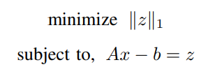
ADMM Solution:

The corresponding Augmented Lagrangian form can be written as,

Combining the y-dependent term into the L2 norm term,

Replacing y/ρ with u (this step can be done anywhere during the solution but is often done to maintain convention),

In order to find the update for x, the minimization of the Lagrangian with respect to x is done as,
Assuming z^k and u^k are known,

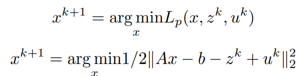
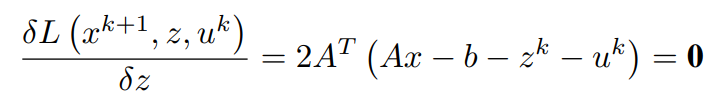
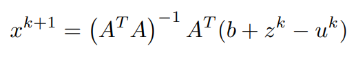
Equating first order partial differential term with respect to x to 0 (0 vectors) and simplifying to obtain x^(k+1)

Similarly, in order to find the update for z, the minimization of the Lagrangian with respect to z is done as,
x^(k+1) has been computed and u^k is assumed to be known,

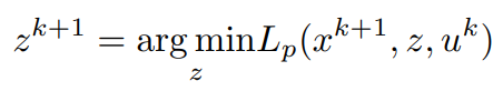
Consider the z-dependent terms,

bringing ρ into a common denominator constant,

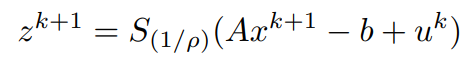
Proximal operator: Consider the proximal operator on a variable v with some constant α to be defined as,

On comparing the latest equation with the proximal operator, the similarity of the Right-hand sides leads us to simplify the obtained z^(k+1) to be represented in a more compact form like,

Both x^(k+1) and z^(k+1) have been computed, using them the update for y can be written as,

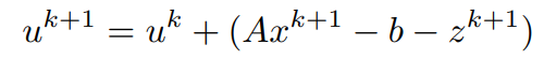
In essence,

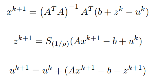
Implementation

A simple and intuitive code implementation of the update steps on synthesised data in Matlab can be done by following the basic steps,

1. Create a toy dataset (possibly linear like the one done below), with this our aim is to verify that the updates are working as intended.
2. Decide upon an objective variable(in the following implementation it would be the variable x0), and add noise to the system, this is to mimic a more realistic observation.
3. Initialize the required variables randomly/to zeros.
4. Code the update equations and loop through them a sufficient number of times/ till convergence.
5. Output the final values obtained by the updates, if done correctly we should observe a relatively close value of the curated and the predicted value obtained from our updates defined by the system.

rand('seed', 0);
randn('seed', 0);

m = 1000; % number of examples
n = 100;  % number of features

% synthesizing required coditions
A = randn(m,n);
x0 = 10*randn(n,1);
b = A*x0;
idx = randsample(m,ceil(m/50));
b(idx) = b(idx) + 1e2*randn(size(idx)); % adding deviations
rho = 1;

% maximum iterations set instead of convergence
MAX_ITER = 1000;

[m, n] = size(A);
x = zeros(n,1);
z = zeros(m,1); 
u = zeros(m,1);
P = inv(A'*A)*A'

for k = 1:MAX_ITER
    % x-update
    x = P*(b + z - u);

    e = A*x;

    % z-update
    z = shrinkage(e - b + u, 1/rho);
    % u-update
    u = u + (e - z - b);
end 

h = {'x0' 'x'};
v = [x0, x];
R = [h;num2cell(v)]
oh = {'z' 'u'};
ov = [z, u];
oR = [oh;num2cell(ov)]

The matlab definition of the assistive function shrinkage is,

function z = shrinkage(x, kappa)
    z = pos(1 - kappa./abs(x)).*x;
end

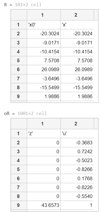
Output

The following output is obtained,

Here,

• x0 represents the synthesized data that we expect to achieve in x with the updates
• and z and u are the corresponding update supportive variable values

Additional code for L1-Norm vs L2-Norm Loss vs Error plot

The following code is in python

import numpy as np
import matplotlib.pyplot as plt

def SE(x,y,intc,beta):
    return (1./len(x))*(0.5)*sum(y - beta * x - intc)**2

def L1(intc,beta,lam):
    return lam*(np.abs(intc)+np.abs(beta))

def L2(intc,beta,lam):
    return lam*(intc**2 + beta**2)

N = 100
x = np.random.randn(N)
y = 2 * x + np.random.randn(N)

beta_N = 10000
beta = np.linspace(-1000,1000,beta_N)
intc = 0.0

L1_array = np.array([L1(intc,i,lam=30) for i in beta])
L2_array = np.array([L2(intc,i,lam=1) for i in beta])

fig1 = plt.figure()
ax1 = fig1.add_subplot(1,1,1)
plt.ylabel("Loss")
plt.xlabel("Error")
plt.grid()
ax1.plot(beta,L1_array,label='L1 norm')
ax1.plot(beta,L2_array,label='L2 norm')
plt.title('The graph of each term of Loss function')
plt.legend()
fig1.show()