LASSO is the acronym for Least Absolute Shrinkage and Selection Operator. Regression models' predictability and interpretability were enhanced with the introduction of Lasso. Therefore, a thorough understanding of mathematics will be useful for ML applications. Using ADMM, we may investigate this solution.
Table of contents
- Introduction
- Machine Learning Context
- Solving the LASSO Problem using ADMM
- Implementation
Introduction
LASSO is often associated with it performing the choices of a smaller set of the known covariates from the data to be used in a model. In other more familiar words, it can be called a Feature Selector.
In general, feature selectors are used to select the most relatively relevant information providing features from all raw observational data.
On carefully reviewing the previous statement we can see that there has to be some logic to deciding on which of the features are considered to be of greater or lesser importance. The simplest way to do this is by manually calculating and comparing the correlation values of each feature of the data vs the result. Before moving further we can look into,
The need for Feature Selectors
The age of digitization has and is producing a tremendous amount of data, to keep up with the amount of data and put it to good use, we employ ML techniques. To feed the models we build with irrelevant features/input would naturally result in it producing corresponding outputs. A well-defined model is one that uses only as many as required features to provide accurate predictions, the advantages of
it are,
- The non-relevant features are not required to be measured or taken into consideration for training the model.
- The possibility of data clutter diminishing the model performance is reduced.
To overcome this issue and to better utilize the models we build we take the help of feature selectors to simplify the task for us.
when the volume of data is scaled, it becomes tedious/almost impossible to manually sort and use the traditional way to decide the features appropriate for the model. LASSO provides an automated solution to this problem.
Machine Learning Context
Let's now establish the same in ML terms. The inspiration for formulating LASSO problem from a machine learning perspective is derived from the following,
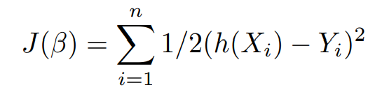
Consider a machine learning model to have ’m’ features and ’n’ data points, conventionally we define the terms in use as,
This model produces predictions using each data point by the function say,

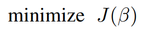
The Cost function J(β) that helps to improve the predictions made by the model is defined as,
here the objective is,
we can now correspondingly modify the objective function to incorporate the decision term. Let's start by considering an L0-Norm,
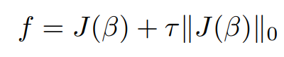
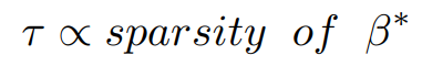
here ∥J(β) ∥0 is a term that describes the number of non-zero terms and τ is the term that defines the strength of consideration
of significant characters, in other words when the value of τ increases then the sparsity of the solution β is increased.
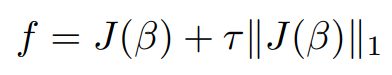
The objective function f(n) from the above equation is intractable i.e., there exist no efficient algorithms to solve it. On replacing
∥J(β)∥0 with equivalent L1 norm ∥J(β)∥1 we obtain,
similarly here the objective is,
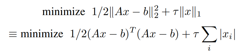
equivalently,

The above equation is the base form and serves as the starting point for the LASSO problem.
Solving the LASSO Problem using ADMM
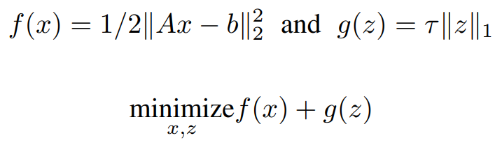
Using a more conventional variable assignment for solving general LASSO problem we can define it as,
Representing the same in ADMM format,
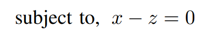
ADMM Solution:
The corresponding Augmented Lagrangian form can be written as,

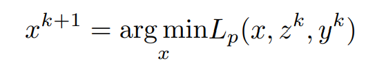
In order to find the update for x, the minimization of the Lagrangian with respect to x is done as,
Assuming z^k and y^k are known,
Consider the x-dependent terms,
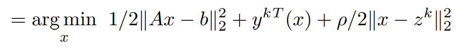
Expanding L2 norm term,

Equating first order partial differential term with respect to x to 0 (0 vectors) and simplifying to obtain x^(k+1)
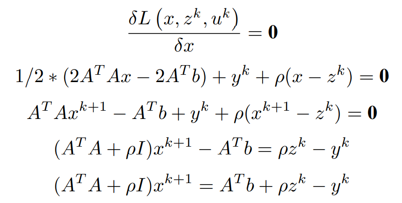
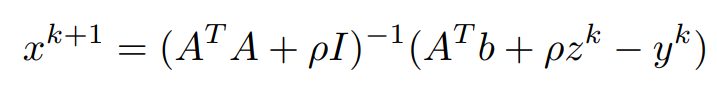
Finally, the x update is obtained as,
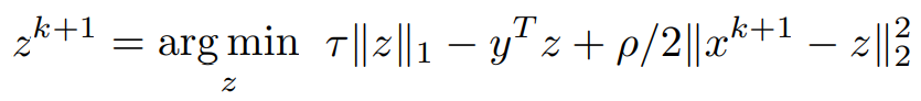
Similarly, in order to find the update for z, the minimization of the Lagrangian with respect to z is done as, x^(k+1) has been computed and y^k is assumed to be known,
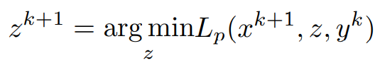
Consider the z-dependent terms,
Pushing the y^Tz term into the L2 norm and dividing by τ
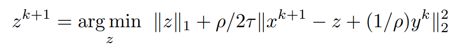
grouping non-z terms,

bringing ρ into a common denominator constant,

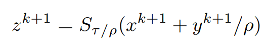
Proximal operator: Consider the proximal operator on a variable v with some constant α to be defined as,

On comparing the above equations, the similarity of the Right-hand sides leads us to simplify the obtained z^(k+1) to be represented in a more compact form like,
Both x^(k+1) and z^(k+1) have been computed, using them the update for y can be written as,
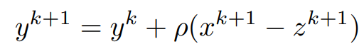
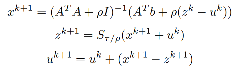
Replacing (1/ρ)y^k with u^k and putting it all together, the updates for each variable are,
Implementation
A simple and intuitive code implementation of the update steps on synthesized data in Matlab can be done by following the basic steps,
- Create a toy dataset (possibly linear like the one done below), with this our aim is to verify that the updates are working as intended.
- Decide upon an objective variable(in the following implementation it would be the variable x0), and add noise to the system, this is to mimic a more realistic observation.
- Initialize the required variables randomly/to zeros.
- Code the update equations and loop through them a sufficient number of times/ till convergence.
- Output the final values obtained by the updates, if done correctly we should observe a relatively close value of the curated and the predicted value obtained from our updates defined by the system.
randn('seed', 0);
rand('seed',0);
m = 1500; % number of examples
n = 5000; % number of features
rho = 100/n; % sparsity density
% synthesizing required conditions
x0 = sprandn(n,1,rho);
A = randn(m,n);
A = A*spdiags(1./sqrt(sum(A.^2))',0,n,n); % normalize columns
b = A*x0 + sqrt(0.001)*randn(m,1); % adding deviations
lambda_max = norm( A'*b, 'inf' );
lambda = 0.1*lambda_max;
% maximum iterations set instead of convergence
MAX_ITER = 1000;
[m, n] = size(A);
% save a matrix-vector multiply
P = inv(A'*A+rho*eye(n))
x = zeros(n,1);
z = zeros(n,1);
u = zeros(n,1);
for k = 1:MAX_ITER
tmp = A'*b + rho*(z - u); % temporary value
% x-update
x = P*tmp;
% z-update
z = shrinkage(x + u, lambda/rho);
% u-update
u = u + (x - z);
end
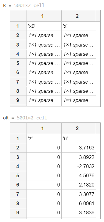
h = {'x0' 'x'};
v = [x0, x];
R = [h;num2cell(v)]
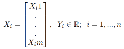
oh = {'z' 'u'};
ov = [z, u];
oR = [oh;num2cell(ov)]
The matlab definition of the assistive function shrinkage is,
function z = shrinkage(x, kappa)
    z = pos(1 - kappa./abs(x)).*x;
end
Output
The following output is obtained,
Here,
- x0 represents the synthesized data that we expect to achieve in x with the updates
- and z and u are the corresponding update supportive variable values