
Huber Fitting in general is the approach of using the Huber function to fit the data models, the advantage of this approach is due to the clever formulation of the Huber function which brilliantly combines the best features of both preceding optimization solution approaches of LAD and LS. To benefit from its theoretical strength, it must therefore be solved in order to acquire a form that can be used in practice. It is advisable to have a solid understanding of ADMM for a better understanding.
Table of contents
- Introduction
- Machine Learning Context
- Solving the Huber Fitting Problem using ADMM
- Implementation
Introduction
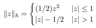
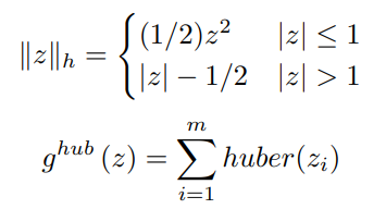
The Huber Loss function is a two piece function defined as follows
We will now examine the incentive for the Huber Loss Function.
Consider the plot of Loss vs Prediction Error for the LAD(labeled as Absolute error), LS(labeled as Squared error) and
Huber Loss,
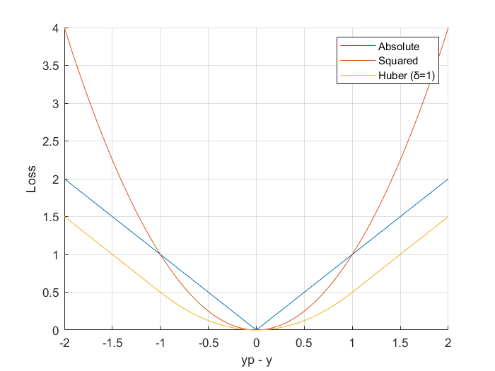
We can observe,
- In the range of values [-δ, +δ] the LS error is lesser than LAD error
- In the range of values (-∞, -δ) ∪ (+δ, +∞) the LAD error is lesser than LS error
From the above observations, we can formulate the Huber loss function that explicitly uses the better performing Errors in both ranges.
Machine Learning Context
The generalized form of Huber loss function often used in ML applications is,
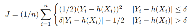
Here,
- Y is the Observed/Actual value
- h(Xi) is the predicted value
Solving the Huber Fitting Problem using ADMM
The Huber Fitting problem can thus be defined as,
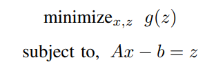
Here, x ∈ R^n, A is a matrix of size mxn and b is a vector of dimension mx1.
ADMM Solution:
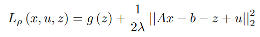
The corresponding Augmented Lagrangian form can be written as,

Replacing y/ρ with u and 1/ρ with λ,
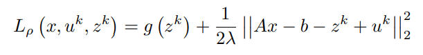
In order to find the update for x, the minimization of the Lagrangian with respect to x is done as,
Assuming z^k and u^k are known,
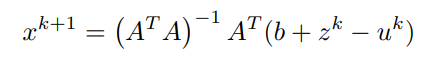
Equating first order partial differential term with respect to x to 0 (0 vectors) and simplifying to obtain x^(k+1)
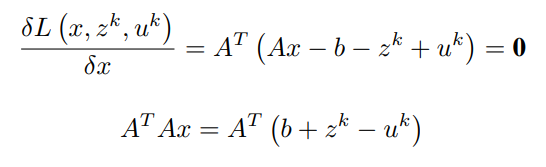
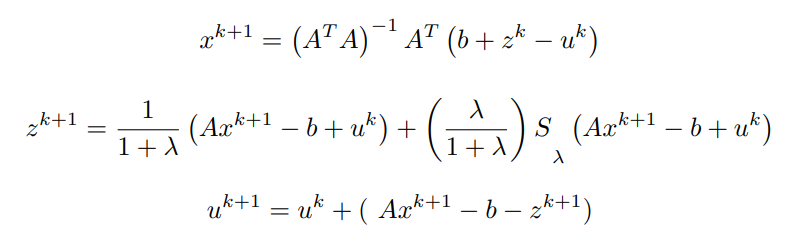
Finally, the update for x is given by,
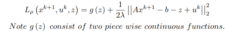
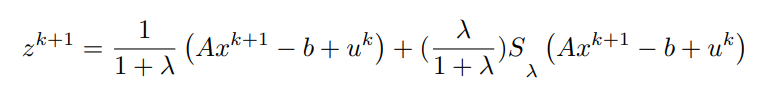
Similarly, in order to find the update for z, the minimization of the Lagrangian with respect to z is done as,
x^(k+1) has been computed and u^k is assumed to be known,
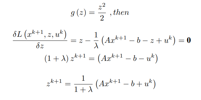
Case – I :
Case – II :
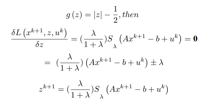
here Sλ represents shrinkage by ±λ sign
We can in turn combine the final equations to get,
Both x^(k+1) and z^(k+1) have been computed, using them the update for y can be written as,
The original Lagrangian multiplier term is u.T
(Ax − b − z)
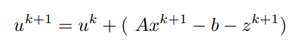
In essence,
Implementation
A simple and intuitive code implementation of the update steps on synthesised data in Matlab can be done by following the basic steps,
- Create a toy dataset (possibly linear like the one done below), with this our aim is to verify that the updates are working as intended.
- Decide upon an objective variable(in the following implementation it would be the variable x0), and add noise to the system, this is to mimic a more realistic observation.
- Initialize the required variables randomly/to zeros.
- Code the update equations and loop through them a sufficient number of times/ till convergence.
- Output the final values obtained by the updates, if done correctly we should observe a relatively close value of the curated and the predicted value obtained from our updates defined by the system.
randn('seed', 0);
rand('seed',0);

m = 5000;  % number of examples
n = 200;   % number of features

% synthesizing required conditions
x0 = sprandn(n,1,rho);
A = randn(m,n);
A = A*spdiags(1./norms(A)',0,n,n); % normalize columns
b = A*x0 + sqrt(0.01)*randn(m,1);
b = b + 10*sprand(m,1,200/m);      % adding sparse, large noise
rho = 1;

MAX_ITER = 1000;
[m, n] = size(A);

% save a matrix-vector multiply
Atb = A'*b;
x = zeros(n,1);
z = zeros(m,1);
u = zeros(m,1);
P= inv(A'*A)

for k = 1:MAX_ITER
    % x-update
    x_new = P*(A'*(b+z-u));

    e  =  A*x_new;
    tmp = e - b + u;

    % z - update
    z_new = rho/(1 + rho)*tmp + 1/(1 + rho)*shrinkage(tmp,1/rho);
    % u - update
    u_new = u + (e - z_new - b);
end

h = {'x0' 'x'};
v = [x0, x_new];
R = [h;num2cell(v)]
oh = {'z' 'u'};
ov = [z_new, u_new];
oR = [oh;num2cell(ov)]
The matlab definition of the assistive function shrinkage is,
function z = shrinkage(x, kappa)
    z = pos(1 - kappa./abs(x)).*x;
end
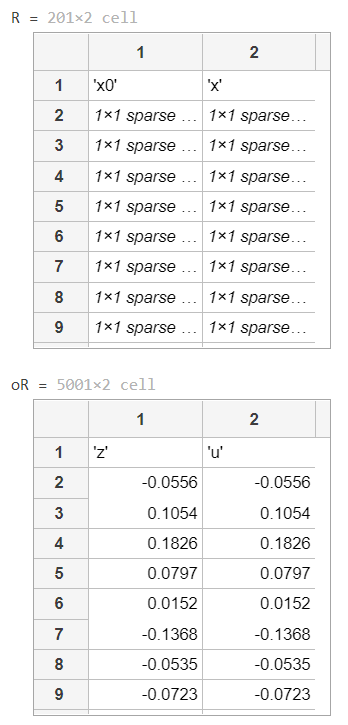
Output
The following output is obtained,
Here,
- x0 represents the synthesized data that we expect to achieve in x with the updates
- and z and u are the corresponding update supportive variable values
Additional code for L1-Norm vs L2-Norm Loss vs Error plot
clc
clear all
close all

x = linspace(-2,2,100);

LAD = abs(x)

LS  = power(x,2)

delta = 1
set_1 = abs(x) <= delta;
set_2 = abs(x) > delta;

Huber = 0.5*set_1.*power(x,2) + set_2.*(abs(x) - 0.5)

hold on
grid on
xlim([-2,2]);
xticks(-2:0.5:2);
ylim([0,4]);
yticks(0:0.5:4);

% Error = actual - predicted
xlabel("yp - y")
ylabel("Loss")
plot(x, LAD)
plot(x, LS)
plot(x, Huber)
legend('Absolute', 'Squared', 'Huber (δ=1)')