In this article, we will cover Pointwise Convolution which is used in models like MobileNetV1 and compared it with other variants like Depthwise Convolution and Depthwise Seperable Convolution.

Table of Contents:

1. Introduction
2. Pointwise Convolution.
   2.1. Application of Pointwise Convolution.
   2.2. Applying Pointwise Convolution.
3. Gradient Backpropagation of pointwise Convolution
4. Pointwise A-trous convolution
5. Running Time
6. Depthwise Convolution vs Depthwise Seperable Convolution vs Pointwise Convolution.

Introduction:

A convolution is the basic process of applying a filter to an input to produce an activation. When the same filter is applied to an input several times, a feature map is created, displaying the positions and intensity of a recognised feature in an input, such as an image.

The capacity of convolutional neural networks to learn a large number of filters in parallel particular to a training dataset within the restrictions of a certain predictive modelling task, such as image classification, is its unique feature. As a result, extremely precise traits appear on input images that may be identified everywhere.

In this article we will discuss about Pointwise Convolution.

Pointwise Convolution:

Pointwise Convolution is a form of convolution that employs a 1x1 kernel, which iterates across each and every point. This kernel has a depth equal to the number of channels in the input picture. It may be used with depthwise convolutions to create depthwise-separable convolutions, which are a useful type of convolution.

Let’s understand pointwise convolution in detail:

The pointwise convolution, which is a convolution operator applied to each point in a point cloud, works as follows:

Each point in a point cloud has a convolution kernel centred on it. Within the kernel support, neighbour points might contribute to the centre point. In each convolution layer, each kernel contains a size or radius value that may be modified to account for the varied number of neighbour points.

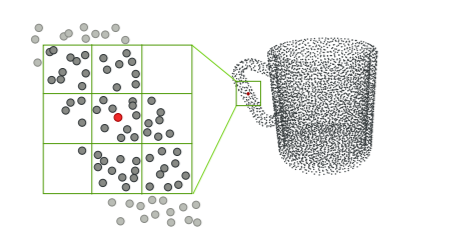
Above Image: Pointwise Convolution

Pointwise convolution can be stated in formal terms as:

where k iterates across all kernel support sub-domains; Ω i(k) is the kernel's kth sub-domain, centred at point i;pi is considered to be the coordinate of point i;|.| wk is the kernel weight at the k-th subdomain, xi and xj the value at point i and j, and ' - 1 and ' the index of the input and output layer, respectively.

Now as we know, pointwise is 1x1 convolution, let's imagine it is applied to M channels, then the filter size of the operation turns out to be 1 x 1 x M and let's imagine we use N filters then the output size will be Dp x Dp x N

Total number of nultiplications for pointwise operation:

Total no of multiplications = M x Dp^2 x N

Application of Pointwise Convolution:

• It may be used with depthwise convolutions to create depthwise-separable convolutions, which are a useful type of convolution.

• To change the input's dimensionality (number of channels).

• Some networks, such as Inception, concatenate features calculated from separate kernels, resulting in an excessive number of channels. To control the number of channels, a pointwise convolution is used.

• Poinwise convolution (basically depthwise separable convolution) is used in models like MobileNet .

Applying Pointwise Convolution:

Before performing pointwise convolution, we need to make the input image go through depthwise convolution.

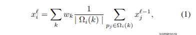
We apply a convolution on the input picture without modifying the depth. We accomplish it by combining three 5x5x1 kernels.

Above Image: Depthwise convolution, uses 3 kernels to transform a 12x12x3 image to a 8x8x3 image

Each 5x5x1 kernel iterates one channel of the picture , obtaining the scalar products of every 25 pixel group, resulting in an image of 8x8x1. When you stack these photos together, you obtain an 8x8x3 image.

The depthwise convolution has currently converted the 12x12x3 picture into an 8x8x3 image. The number of channels in each picture must now be increased.

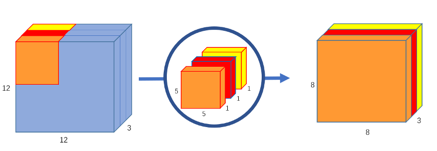
Now performing Pointwise Convolution:

To generate an 8x8x1 image, we cycle a 1x1x3 kernel across our 8x8x3 picture.

Above Image: Pointwise convolution, transforms an image of 3 channels to an image of 1 channel

To produce a final picture of shape 8x8x256, we can build 256 1x1x3 kernels that individually output an 8x8x1 image.

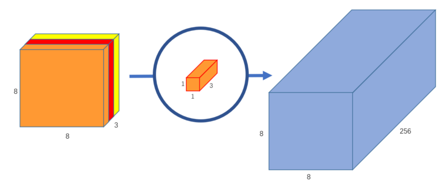
Above Image: Pointwise convolution with 256 kernels, outputting an image with 256 channels

And We’ve separated the convolution into a depthwise convolution and a pointwise convolution.

Gradient Backpropagation of pointwise Convolution:

For making pointwise convolution trainable, the gradients with respect to the input data and kernel weights must be computed. The loss function is denoted by the letter L. In terms of input, the gradient might be described as:

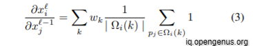
where we iterate over all neighbor points i of a given point j. In the chain rule, ∂L/∂x i is the gradient up to layer , which is known during back propagation. The derivative ∂x i /∂x −1 j could be written as:

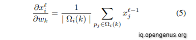
Similarly, the gradient in kernel weights may be determined by iterating over all locations/points i:

Where,

Pointwise A-trous convolution:

By incorporating a stride parameter that defines the spacing between kernel cells, the basic pointwise convolution may simply be expanded to a-trous convolution. The advantage of pointwise a-trous convolution is that it allows you to increase the kernel size, and therefore the perceptive field, without having to process too many points. This results in considerable speed gains without losing accuracy.

Running Time:

One of the most difficult aspects of implementing pointwise convolution is determining how to execute rapid nearest neighbour queries without significantly slowing down network training and prediction. A grid for neighbour query is employed to make the training possible since it is a lightweight and GPU-friendly data structure to generate and query on the fly. In reality, kd-tree was tried, but it was discovered that on contemporary CPUs and GPUs, a kd-tree query does not outperform a grid till the number of points is greater than 16K, not to mention the extra time required for tree building, which has an O(n log n) complexity.

On an Intel Core i7 6900K with 16 threads, forward convolution of our network takes 1.272 seconds, while backward propagation takes 2.423 seconds to compute the gradients for a batch size of 128 point clouds, each with 2048 points. On an NVIDIA TITAN X, GPU implementation can improve the running time by around ten percent.

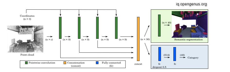
Above Image: Pointwise convolutional neural network

Depthwise Convolution vs Depthwise Seperable Convolution vs Pointwise Convolution:

Depthwise Convolution:
Depthwise Convolution is a sort of convolution in which each input channel receives a single convolutional filter. The filter is as deep as the input in normal 2D convolution conducted over multiple input channels, allowing us to arbitrarily combine channels to produce each element in the output.

Depthwise Separable Convolution:
Kernels that cannot be "factored" into two smaller kernels are used in depthwise separable convolutions. As a result, it is more widely utilised. A depthwise separable convolution separates a kernel into two independent kernels, each of which performs two convolutions: the depthwise and pointwise convolutions.

Pointwise Convolution:
The pointwise convolution gets its name from the fact that it utilises a 1x1 kernel, which iterates across every single point. This kernel has a depth equal to the number of channels in the input picture.

With this article at OpenGenus, you must have the complete idea of Pointwise Convolution.