
Any person who would have seen the MobileNet architecture, would have stumbled across the term separable convolution. What is separable convolution and how is it different from regular convolution?
Table of Content:
- Spatial separable convolution
1.1 Spatial separable convolution - An example
1.2 Spatial separable convolution - Mathematics behind computational cost
1.3 Conclusion - Depthwise separable convolution
2.1 Depthwise separable convolution - An example
2.1.1 Depthwise convolution
2.1.2 Pointwise convolution
2.2 Depthwise separable convolution - Mathematics behind computational cost
2.3 Conclusion - Alternatives to separable convolution
Separable convolution comes in two types:
- Spatial separable convolution
- Depthwise separable convolution.
We shall discuss about both in this article.
1. Spatial separable convolution
Spatial separable convolution is the easier of the two so we'll disuss it first. The spatial separable convolution works on the spatial features of an image: its width and its height. These features are the spatial dimensions of the image hence the name, spatial separable. It decomposes the convolution operation into two parts and applies each separated convolution in succession. For instance, the Sobel filter (or the Sobel kernel), which is a 3x3 filter is split into two filters of size 3x1 and 1x3.
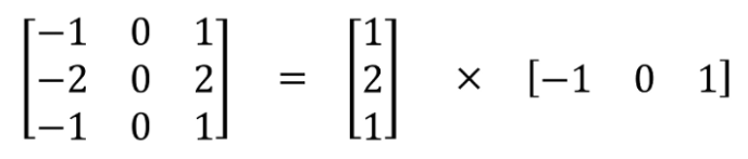
As you can see, the 3x3 filter is spilt into a 3x1 and a 1x3 filter. The output does not change as the image still obeys the matrix multiplication rule. The image when the 3x1 filter is applied will have the column dimension as 1 which is the row dimension of the next filter, the 1x3 filter. What is changed is the number of multiplications that are performed. Spatial separable convolution reduces the number of individual multiplications.
In a regular 3x3 convolution, there are a total of 9 operations. But when we split the matrix into a 3x1 and a 1x3 filter, there are a total of 6 operations. Therefore, less matrix multiplications are needed when convolving it in an image.
1.1 Spatial separable convolution - An example
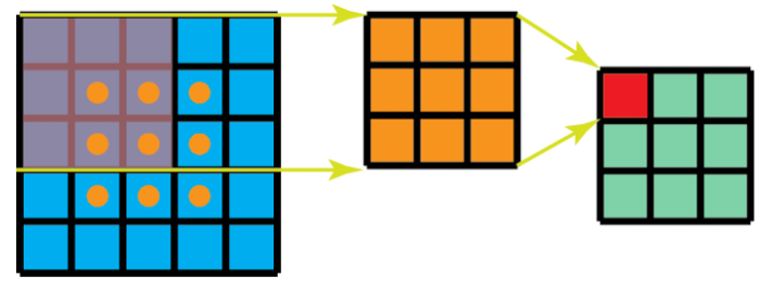
Take an example of a 5x5 image with a 3x3 kernel convolving with a stride of 1 and 0 padding. The 3x3 kernel would scan at 3 positions horizontally and 3 positions vertically making the total of 9 positions. The 9 positions are shown in the image below. At each point, a total of 9 matrix multiplication (element-wise) would be applied bringing a total of 9 x 9 = 81 total multiplications.
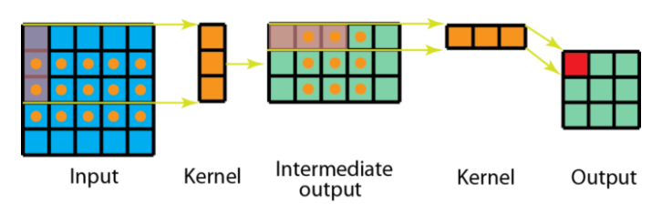
Now, consider the spatial separable convolution in action. We apply the 3x1 filter first on the 5x5 image. By scanning 5 horizontal positions and 3 vertical positions, we get a total of 3 x 5 = 15 positions. These positions are shown in the 5x3 intermediate matrix. At every position, rather than having 9 element-wise matrix multiplication, we only have 15 x 3 = 45 multiplications. But that is not the final matrix. The intermediate 5x3 matrix is then convolved with the 1x3 filter, scanning the matrix at 3 positions horizontally and 3 positions vertically. We get a total of 3 x 3 = 9 positions in which, after applying 3 element-wise matrix multiplication, brings a net 9 x 3 = 27 total matrix multiplications. Thus, our total adds up to 45 + 27 = 72 multiplications. That is a reduction of 9 whole element-wise matrix multiplication. The respective positions are marked in the figure below.
1.2 Spatial separable convolution - Mathematics behind computational cost
Let's generalize the formula. For any N x N image, applying convolutions with an m x m kernel having stride of 1 and padding of 0:
- Traditional convolution requires ((N - 2) x (N - 2) x m x m) matrix multiplications.
- Spatially separable convolution requires (N x (N-2) x m) + ((N-2) x (N-2) x m) = (2N-2) x (N-2) x m multiplications.
We can find the ratio of computation costs between both the approaches. The ratio between computational cost of spatial separable convolution and computational cost of regular convolution is:
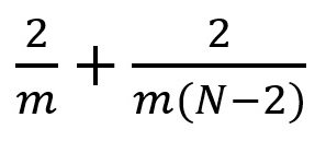
We can see this ratio becomes 2 / m when the image size is way larger than the filter size (when N >> m). Putting values of kernel size, m = 3, 5, 7, and so on, we see that the computational cost of spatially separable convolution is 2/3 (about 66%) of the standard convolution for a 3 x 3 filter, 2 / 5 (40%) for a 5 x 5 filter, 2 / 7 (about 29%) for a 7 x 7 filter, and so on.
1.3 Conclusion
We see that spatial separable convolution saves the overall cost by having less number of matrix multiplications. Still, why is it not used extensively in deep learning applications? The main reason is that not all convolutional filters (kernels) can be decomposed (or separated) into two smaller kernels. Further, by replacing all conventional convolutional kernels with spatailly separable kernels, we might limit ourselves for searching all possible kernels during training resulting in sub-optimal training results.
2. Depthwise separable convolution
Moving on to the next type of separable convolution, depthwise separable convolution are used with filters that cannot be decomposed into smaller filters. Thus, it is more prevalent in most deep learning architectures. MobileNet and Xception are two such examples where depthwise separable convolution is used. We see this separable convolution in Keras (as keras.layers.SeperableConv2D) as well as in Tensorflow (as tf.layers.separable_conv2d).
Deptwise separable convolution, unlike spatial separable convolution, also deals with the depth dimension as well. The depth dimension refers to the number of channels an image has. We know that any image has 3 different channels, RGB, which tell the "redness", "greenness" and "blueness" of each pixel. Depthwise separable convolution works in a similar way as spatial separable convolution: the kernel is split into 2 different kernels known as the depthwise convolution and the pointwise convolution. We shall see how this works by taking an example.
2.1 Depthwise separable convolution - An example
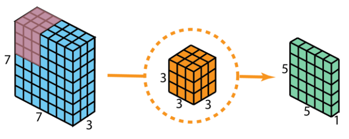
We consider our input layer to be of size 7 x 7 x 3 (height x width x channels). Our filter size is 3 x 3 x 3. We apply regular 2D convolution first as a sort of comparison. After applying 2D convolution with just one filter, we get a 5 x 5 x 1 output layer having only 1 channel. Figure below illustrates this well.
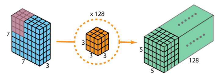
As many of you may know, numerous filters are applied between any two neural network layers. Let's say, for example purposes, that we have 128 filters. After performing 128 2D convolutions, we get a total of 128 5 x 5 x 1 output layers. Let's stack all these layers into a big layer; that layer will have a size of 5 x 5 x 128. We are able to shrink the spatial dimensions which are the height and width (from 7 x 7 to 5 x 5). However, the depth increased from 3 layers to 128.
As we did in the spatial separable convolution (see section above), let's find the number of multiplications required with the tradiational approach. We have 128 3 x 3 x 3 filters moving 5 x 5 times. Multiplying the filters with the moving done, we get 128 x 3 x 3 x 3 x 5 x 5 = 86,400 multiplications.
Let's see how depthwise separable convolution achieves the similar result.
2.1.1 Depthwise convolution
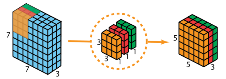
With the same example as above, we first apply depthwise convolution (recall that this approach uses depthwise and pointwise convolution; it is discussed in the introductory part of this section). We use three seperate kernels of size 3 x 3 x 1 instead of using just one 3 x 3 x 3 used in the traditional 2D convolution kernel. The three kernels interacts (convolves) with just one channel of the input layer. Each of these three convolutions produces a map of size 5 x 5 x 1. Perform stacking again to generate a map of size 5 x 5 x 3. We observe that the spatial dimensions have shrunk while the depth remains the same.
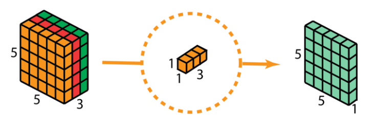
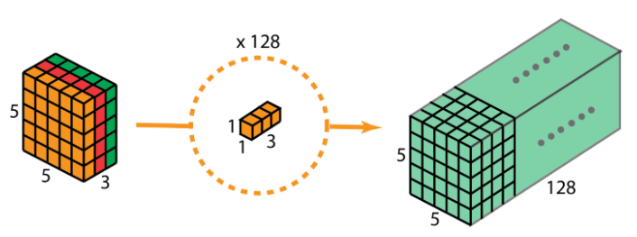
2.1.2 Pointwise convolution
The pointwise convolution is next. With our 5 x 5 x 3 as the input, we apply 1 x 1 convolution having filter size as 1 x 1 x 3. This gives us the same 5 x 5 x 1 output as earlier.
Recall that there are multiple filters are applied between any two neural network layers. We took 128 such filters. So, after applying 128 1 x 1 convolutions, we get the output layer with size 5 x 5 x 128, same as we got in the traditional approach.
To get a whole picture of depthwise separable convolution, refer to the figure below.
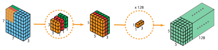
Let's talk numbers now, shall we. How much faster is the depthwise separable convolution? Well it turns out, quite a lot faster! Here is how the math breaks down. Performing depthwise convolution, we have 3 3 x 3 x 1 filters moving 5 x 5 times, bringing a total of 3 x 3 x 3 x 1 x 5 x 5 = 675 multiplications. In pointwise multiplication, we have 128 1 x 1 x 3 filters moving 5 x 5 times, making a total of 128 x 1 x 1 x 3 x 5 x 5 = 9,600 multiplications. This brings us a total of 675 + 9600 = 10,275 multiplications, a mere 12% of the total cost of the traditional 2D convolution!
2.2 Depthwise separable convolution - Mathematics behind computational cost
Let's generalilze the formula. For an input image of size H x W x D, we want to do 2D convolution with stride=1 and padding=0 having Nc kernels of size h x h x D, where h is even. The above convolution transforms the input layer into the output layer of size H-h+1 x W-h+1 x Nc. Thus,
- Traditional 2D convolution requires Nc x h x h x D x (H-h+1) x (W-h+1) multiplication.
- Depthwise seperable convolution requires D x h x h x 1 x (H-h+1) x (W-h+1) + Nc x 1 x 1 x D x (H-h+1) x (W-h+1) = (h x h + Nc) x D x (H-h+1) x (W-h+1) multiplications.
The ratio of computational cost between the two approaches is:
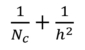
For modern architectures, Nc >> h reducing the equation to be 1/h^2. With this asymptotic notation, a 2D convolution spend 9 times more multiplications when having 3 x 3 filters. For 5 x 5 filters, 2D convolutions spend 25 times more multiplications.
2.3 Conclusion
That is all the good news. Is there any limitations to use depthwise separable convolutions? Well it turns out, depthwise separable convolutions reduce the number of parameters in the convolution. Thus, small models might give sub-optimal results if depthwise separable convolution is used in place of traditional 2D convolution. If used wisely, depthwise separable convolution can actually be efficient without affecting model's performance.
3. Alternatives to separable convolution
While separable convolution is one of many convolution techniques out there, one can choose from a list of different convolution techniques that specialize in specific domains. Alternatives to separable convolution includes:
- Transposed Convolution (Deconvolution, checkerboard artifacts)
- Dilated Convolution (Atrous Convolution)
- Flattened Convolution
- Grouped Convolution
- Shuffled Grouped Convolution
- Pointwise Grouped Convolution
With this article at OpenGenus, you must have the complete idea of Separable Convolution which is used in MobileNetV1 model. Enjoy.