
In this article, we have explored Swish Activation Function in depth. This was developed by Researchers at Google as an alternative to Rectified Linear Unit (ReLu).
Table of contents:
- Overview of Neural Networks and the use of Activation functions
- Swish Activation function
- Derivative function of Swish
- Conclusion
Pre-requisite: Types of Activation Functions used in Machine Learning
Overview of Neural Networks and the use of Activation functions
The mechanism of neural networks works similarly to human brains. When the neural network is fed with a lot of data, it tries to separate useful from useless data much like how human brains work. Activation functions are the algorithms that the neurones use to sort out useful data from useless data. Activation functions basically determine the output of a function based on the input. So, if the input itself is useless and the algorithm can’t make sense of the input, then the output is consequently useless as well. In some cases, you will have dead neurones when they are saturated, this is when there is little or no variation in the outputs based on the nature of the inputs and the activation function used. This saturation means all outputs will be relatively equal making subsequent outputs not-so-useful. Saturation, and dead neurones make it hard for the models to learn during back propagation.
Since I have introduced a term propagation, I think it is necessary to give a brief explanation for what it is. Propagation in AI is just the flow of sequences for making decisions and learning. There is forward propagation and backward propagation. Forward propagation is from the input layer to the output layer. This is the process of the model doing what it was designed to do (ex. making a prediction). It does this by processing information from layer to layer, and each layer has a set of neurones with activation functions, that give an output to the neurones in the subsequent layer. Backward propagation is from the output layer to the input layer. This is the process for the model to learn the steps taken to arrive at a prediction. If it is a right prediction the model learns it to be able to use when a similar situation arises. When it is a wrong prediction, an error is calculated and back propagation will find ways to correct the decisions made to arrive at the wrong prediction. It does this by calculating the differential of the error compared to the differential of the activation functions in each neurone on each layer to optimise their outputs. Back propagation processes the derivatives of the activation functions and hence why learning is harder with dead/saturated neurones.
In this article, we will talk about the Swish activation function and how it works. See this article ELU for the description of another activation function (Exponential Linear Unit - ELU).
Swish Activation function
The most widely used activation function is the Rectified Linear Unit (ReLu) which is defined by,
f(x) = max(0,x); hence the output is never less than 0.
Click the following link for ELU: Exponential Linear Unit
Researchers at google wanted to bridge the gap between the ease of computation of the ReLu and the performance on much deeper datasets. Hence the swish function was developed, which is defined by,
swish(x)=f(x)=x*sigmoid(βx); where β is a scalable and trainable constant.
sigmoid(x)=σ(x)= 1/(1+e^(-x))
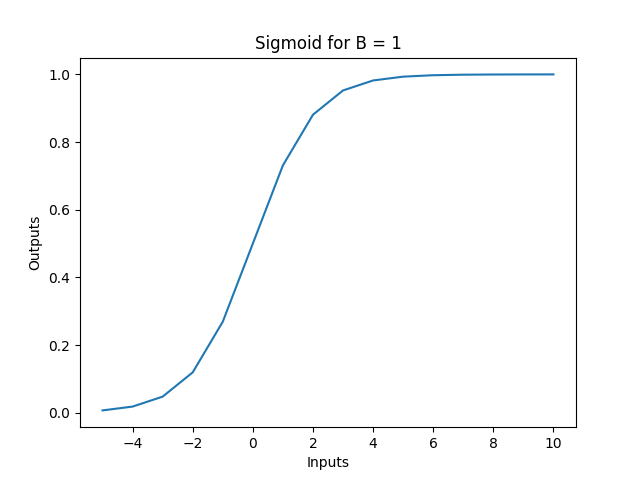
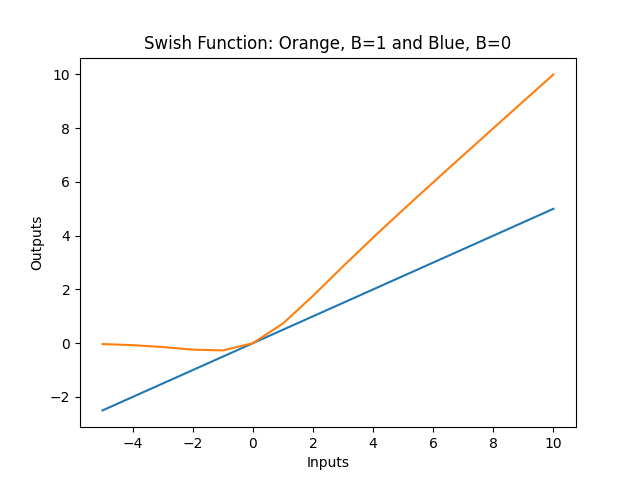
When β = 1, the swish function becomes a simple sigmoid-weighted linear unit function. But when β = 0 then the swish function simply scales the input by 1/2 . The limit as β → ∞, or -∞ of the sigmoid function component returns 0 or 1 based on the value of x (i.e. 1/(1+0)=1/1 = 1 , or 1/(1+∞)=1/∞=0 ). Hence the swish function is a nonlinear function serves to allow the features of linear functions and ReLu functions to work together. The degree at which they can interact is based on the value of β, and this can be controlled by the model if you declare β as a trainable parameter so that the model will learn to optimise it.
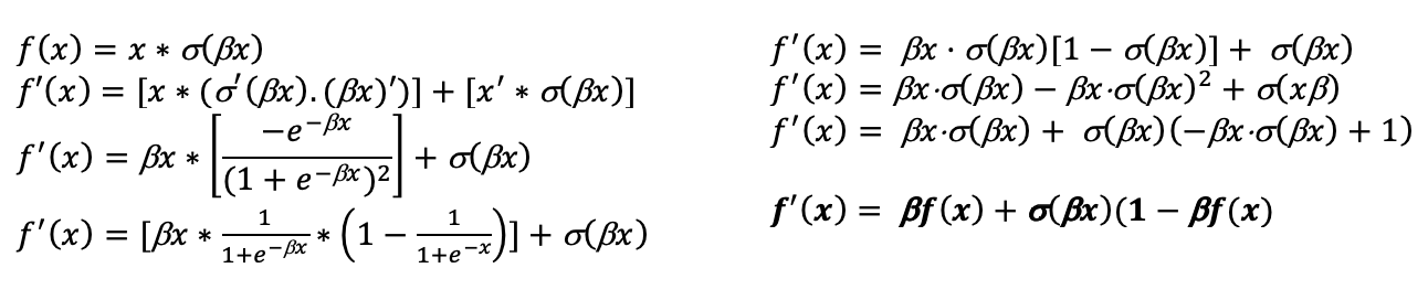
Derivative function of Swish
Like we’ve already discussed, the derivatives of activation functions are needed during back propagation as the differential of the error is compared to the differential of the outputs of each node to optimise these outputs for a better error value or to learn these outputs if the error value is 0(i.e., the prediction was correct).
Given;
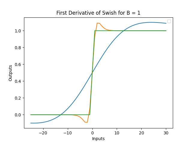
Below is the graph of the first derivatives of a swish function with arbitrary x inputs from -25 to 30 and β as 0.1, 1 and 10. Notice that all three graphs are bounded from 0 to 1, and the value of β chosen dictates how fast the graph reaches these horizontal asymptotes.
Conclusion
The swish function was discovered by google researchers looking for an activation function for deep datasets with the computational simplicity of the ReLu function and the efficiency of results. The swish function reports more efficient results on multiple datasets compared to other activation functions when is set as a trainable parameter (See more about Swish compared to other activation functions here).
See below for the code for the swish and sigmoid functions. Feel free to play with the input values and the values to understand the function better.
import numpy as np
import matplotlib.pyplot as plt


def sigmoid(b, x):
    sig = 1 / (1+np.exp(-b*x))
    return sig


def swish_function(b, x):
    swish = x * sigmoid(b, x)
    return swish


def swish_derivative(b, x):
    swish_der = (b*swish_function(b, x)) + (sigmoid(b, x)*(1-(b*swish_function(b, x))))
    return swish_der


for b in [0, 1]:
    inputs = [x for x in range(-25, 31)]
    output = [swish_function(b, x) for x in inputs]
    plt.plot(inputs, output, label="swish_function")

# b_s = [0.1, 1, 10]
# for b in u_s:
#     inputs = [x for x in range(-25, 31)]
#     output_swish_der = [swish_derivative(b, x) for x in inputs]
#     plt.plot(inputs, output_swish_der, label="first derivative of swish function")

# b = 1
# inputs = [x for x in range(-25, 31)]
# output_sig = [sigmoid(b, x) for x in inputs]
# plt.plot(inputs, output_sig, label="sigmoid function")


plt.ylabel("Outputs")
plt.xlabel("Inputs")
plt.title("Insert Title Here...")
plt.show()
With this article at OpenGenus, you must have the complete idea of Swish Activation function.