
Get this book -> Problems on Array: For Interviews and Competitive Programming
In this article, we will see how time series forecasting is done using Python. We have forecasted / predicted the stock market trends of HDFC using NIFTY50 stock market data.
Table of contents
- Exploring the dataset
- Checking for stationarity
- Making the time series stationary
- Deciding our ARIMA model
- Creating the ARIMA model
Exploring the dataset
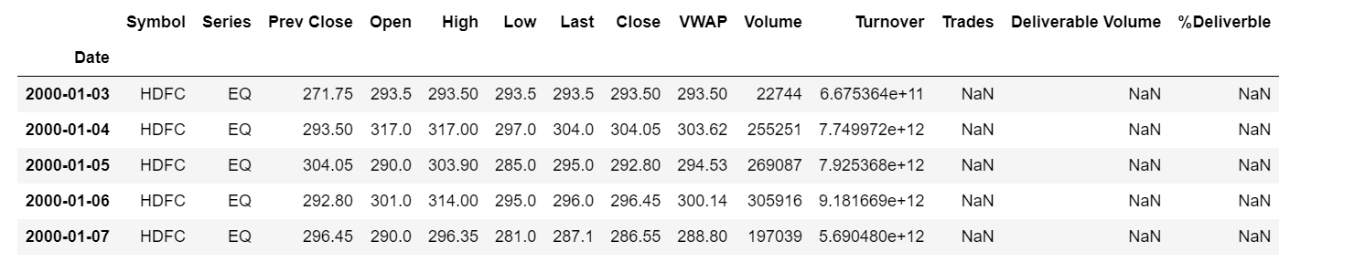
In this tutorial, we will be forecasting the stock market trends of HDFC with the help of an ARIMA model. The dataset used can be found here: NIFTY50 Stock Market data. As our first step, we load the dataset into our environment and see what it looks like. The code snippet is given below.
import pandas as pd
import matplotlib.pyplot as plt
df=pd.read_csv(r'HDFC.csv',index_col='Date',parse_dates=True)
df.head()
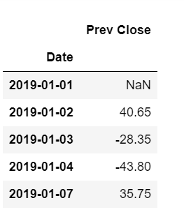
The given code speaks for itself. It just reads our csv file and then displays the first 5 entries of our dataset. Note that we give 'parse_dates=True' while we read our dataset to make sure that python understands that we are dealing with dates. By default, dates are read as strings. But this makes sure that it is read as DateTimeIndex values. The head of our dataset looks like:
Then we get the shape of our dataset.
df.shape
Output:
(5306, 14)
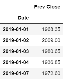
For the purpose of simplicity, we are going to just consider one column 'Prev Close' for the year 2019. And as a part of cleaning the dataset, we are going to drop rows with null values in them.
df=df.dropna()
df=df['Prev Close']['2019-01-01':'2019-12-31']
df=pd.DataFrame(df)
df.head()
Now the head of the dataset looks like:
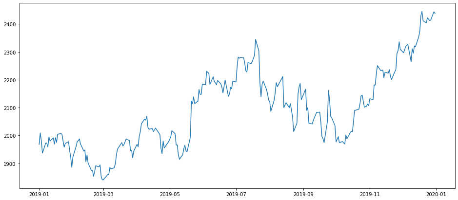
Let us now plot our data to get a better understanding of it.
plt.figure(figsize=(16,7))
plt.plot(df)
plt.show()
Checking for stationarity
With just a look at our plot, we can see that the data is not stationary. Just to confirm it, we perform an Augmented Dickey Fuller (ADF) test to check the stationarity of the data. To perform an ADF test, we import the following module.
from statsmodels.tsa.stattools import adfuller
Then we define our test as a function.
def ad_test(dataset):
     dftest = adfuller(dataset, autolag = 'AIC')
     print(" P-Value : ", dftest[1])
     print(" ADF : ",dftest[0])
     print(" Critical Values :")
     for key, val in dftest[4].items():
         print("\t",key, ": ", val)
And finally, we run the test on our data.
ad_test(df)
Output:
 P-Value :  0.7683096329675532
 ADF :  -0.9578955907704426
 Critical Values :
	 1% :  -3.457437824930831
	 5% :  -2.873459364726563
	 10% :  -2.573122099570008
Out of all the numbers shown, we are only concerned about one number: P-value. This determines the stationarity of our data.
- If p-value is < 0.05, then data is stationary.
- If p-value is > 0.05, then data is non-stationary.
Now, the p-value of our data is 0.76 which is way greater than 0.05. Hence our data is non-stationary.
Making the time series stationary
To make our time series stationary, we use differencing. It helps reduce seasonality, trends and stabilizes the mean. Differencing subtracts the value of a row from the previous row's data and assigns it to that row. The first difference of a time series is the series of changes where the difference in period is 1. If Yt denotes the value of the time series Y at period t, then the first difference of Y at period t is equal to Yt-Yt-1.
The code snippet is as follows:
df1=df.diff(periods=1)
plt.figure(figsize=(16,7))
plt.plot(df1)
plt.show()
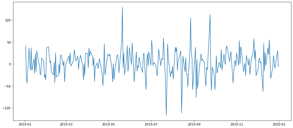
We can observe from the above graph that the mean of our data remains almost the same and hence it is stationary.
The head of our data now looks as:
df1.head()
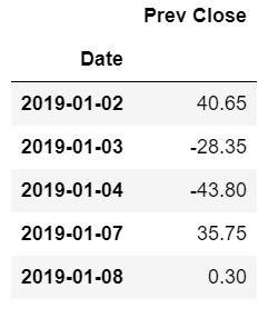
Since the first is a null value, we remove it.
df1=df1[1:]
df1.head()
To confirm stationarity, we will again perform an ADF test on the differenced data.
ad_test(df1)
Output:
 P-Value :  9.826294849897782e-18
 ADF :  -10.114123554614096
 Critical Values :
	 1% :  -3.4577787098622674
	 5% :  -2.873608704758507
	 10% :  -2.573201765981991
Now our p-value is < 0.05 , which means our data is stationary.
Deciding our ARIMA model
Our ARIMA model takes in three values (p,d,q). These are the orders of the respective models. Here,
- p is the order of the auto-regressive (AR) model.
- d represents the 'I' or integrated part and it signifies the difference order. For stationary data, it is usually 0.
- q is the order of the moving average (MA) model.
Since we have differenced our data once, it is first order difference. Hence the value of d is 1. For finding the values of q and p, we use autocorrelation and partial autocorrelation plots.
import statsmodels.api as sm
plt.rcParams['figure.figsize']=(12,8)
fig,axs=plt.subplots(2,1)
fig1=sm.graphics.tsa.plot_acf(df1.dropna(),lags=40,ax=axs[0])
fig2=sm.graphics.tsa.plot_pacf(df1.dropna(),lags=40,ax=axs[1])
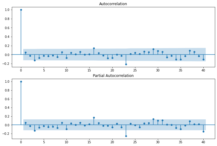
The highlighted areas in the plots represent the confidence intervals. By default, it is set to 95%. To calculate the value of q, we look at our autocorrelation plot. Within the confidence interval, the pointer that first touches or crosses the boundary is taken as the value. In our autocorrelation plot, we find that the third pointer is the first to cross the boundary. Hence the value of q is 3.
Similarly, for getting the value of p, we look at the partial autocorrelation plot. The procedure is same as given above. Hence the value of p too is 3.
Now, we got the (p,d,q) values for the best-fit ARIMA model. They are (3,1,3). Instead of plotting graphs to find values, we can also make use of the 'auto_arima' function in the pmdarima module.
Creating the ARIMA model
To build our ARIMA mode, we import the following.
from statsmodels.tsa.arima_model import ARIMA
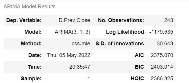
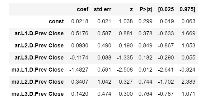
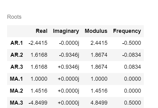
Then we create our model, fit the values in it and obtain the model summary.
model=ARIMA(df1,order=(3,1,3))
model_results=model.fit(disp=-1)
model_results.summary()
We plot the predictions and the original data to check the accuracy of prediction.
plt.plot(df1,label='original')
plt.plot(model_results.fittedvalues,color='red',label='ARIMA prediction')
plt.legend(labels=['original','ARIMA prediction'])
plt.show()
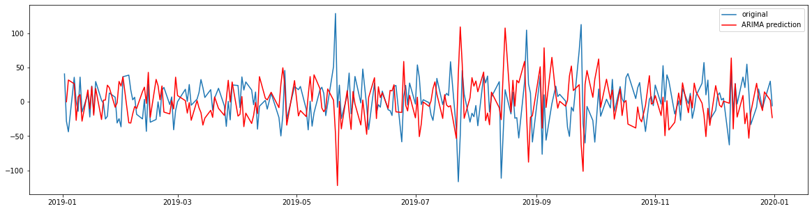
We can see that our model captured the trend of the original data pretty well. Now, we convert the predicted results to the original format i.e we reverse the differencing done on data.
ARIMA_diff_pred=pd.Series(model_results.fittedvalues,copy=True) # converting the fitted values of the results into series
ARIMA_pred_cumsum=ARIMA_diff_pred.cumsum() # calculating the cumulative sum
ARIMA_pred=pd.Series(df1.iloc[0],index=df1.index)
ARIMA_pred=ARIMA_pred.add(ARIMA_pred_cumsum,fill_value=0) # adding the cumulative sum to the differenced data to cancel out the differencing effect
Now, we plot the results and original data again to see the final prediction.
plt.plot(df1,label='original')
plt.plot(ARIMA_pred,color='red',label='ARIMA prediction')
plt.legend(labels=['original','ARIMA prediction'])
plt.show()
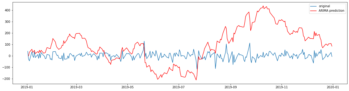
We can see that our model can be improved even though it captures the trend. This can be done by using different transformations on the data and tuning the hyperparameters of the model.