Basics of Time Series Prediction

In simple terms, time series is a series when the index is time such as element at time=1, element at time=2 and so on. In reality, several data can be modeled as a time series data like stock prices (prices vary with time), weather forecasts, Moore's law (Number of chips over time) and much more. Time series prediction is the task where the initial set of elements in a series is given and we have to predict the next few elements. These are significant as it can be used to predict video frames as well when provided with initial frames.

Time series is of two types:

• Univariate
• Multivariate

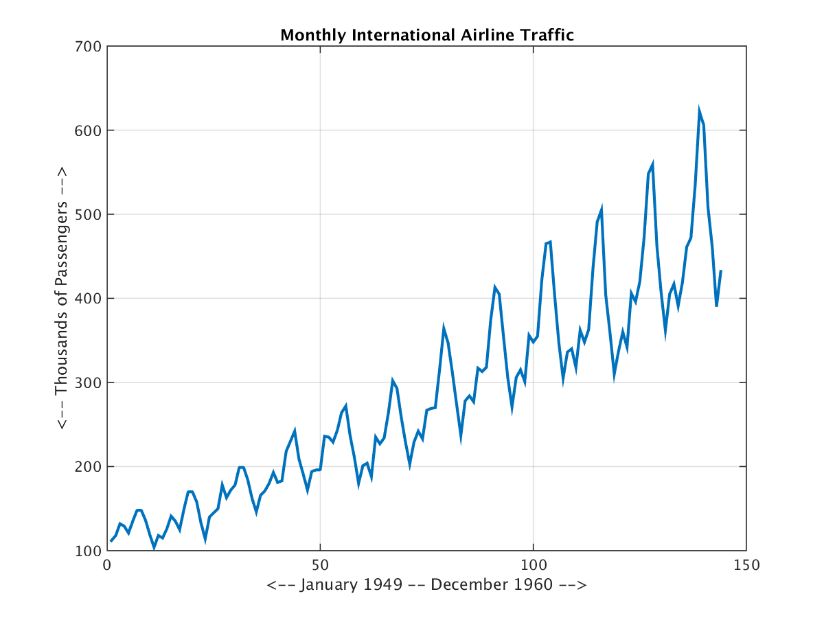
Univariate time series data is a series where only a single parameter changes with time. Examples of such a series are stock prices (only stock changes with time), weather forecast (only weather changes with time) and many other.

Example of Univariate time series data:

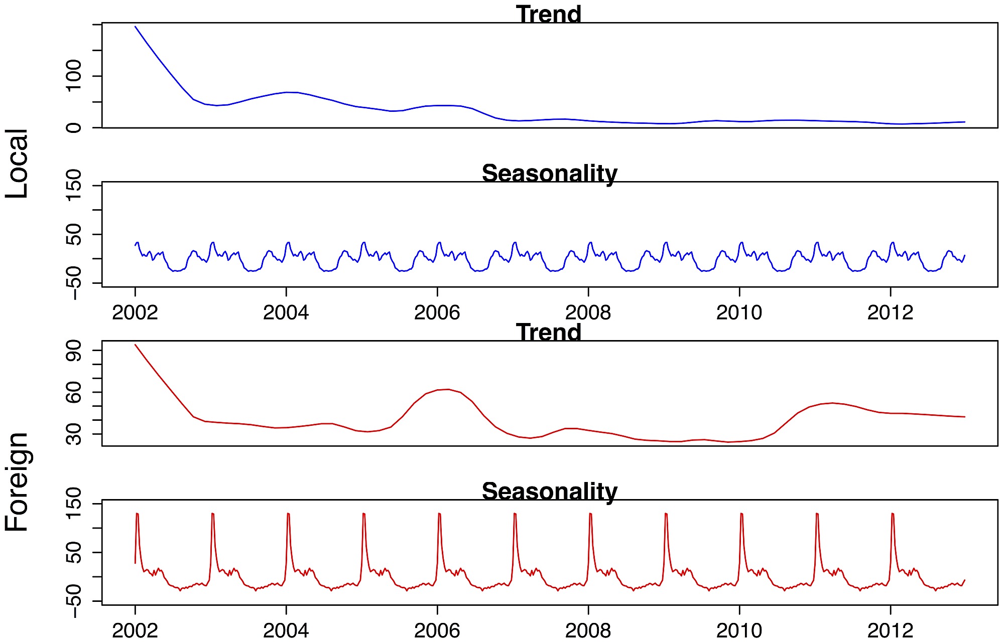
Multivariate time series have multiple values at each time step. These are used when you have multiple data varying with time in a series such as market and sales analysis, temperature and humidity analysis , birth and death rate of a specific region etc.

Time series comes in all shapes and sized but there are some common patterns that we usually see in time series. Such patterns are:

• Trend where time series have a specific direction they are moving in. It is a upward trend when the overall slope of the series is increasing. When the slope is decreasing it's downwards trend. Trend helps us analyze the data well. In the following plot series have a downward trend as it's slope is negative and decreasing with time.

• Seasonality is seen in time series data when patterns repeat at predictable intervals. It follows a very regular patterns in the time series which can be seen clearly. The seasonality can be clearly seen in the time series given below. The particular pattern repeat after certain intervals.

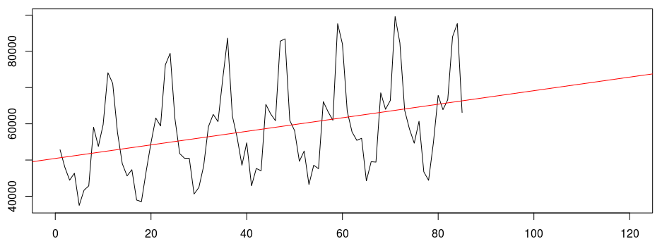
• Trend plus seasonality is a common pattern that can be seen in time series. In this time series have a overall trend but there are local peaks and troughs forming a seasonality in series. This is a combination of trend and seasonality pattern. The following time series have an overall upward trend but there is seasonal pattern also present.

• Auto-correlation: In this entire series isn't random, there are spikes in the time series data. Between the spikes there is a very deterministic type of decay. It correlates with a delayed copy of itself often called a lag. The spikes which cannot be predicted on previous are called innovations.
  By contrast, correlation is simply when two independent variables are linearly related.

Train, Validation and test sets in Time series data

Time Series forecasting is the use of a model to predict future values based on previously observed values. Time series are widely used for non-stationary data, like economic, weather, stock price, and retail sales in this post. To measure the performance of our forecasting model, we typically want to split the time series into a training period, validation period and test period. It can be done in two ways fixed part training and roll forward partitioning.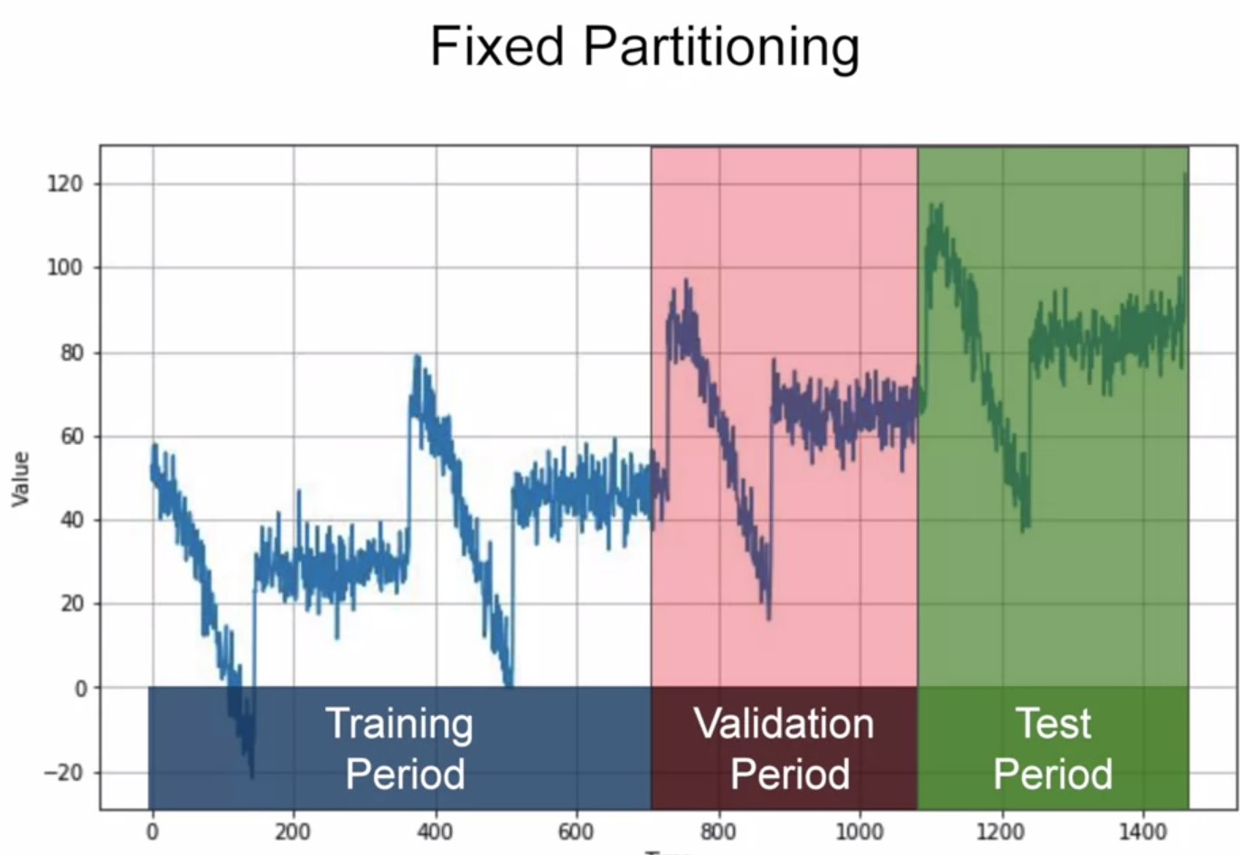
You generally have to ensure that each period contains a whole number of seasons. You will train your model on train period, and work on it and your hyper parameters until you get the desired performance, measured using the validation set. Often, once we're done with training and validation then you can retrain using both the training and validation data and then test on the test period to see if your model will perform just as well and if it does, then you could take unusual step of retraining again, using also the test data. But why would we do that? Well, it's because the test data is the closest you have to the current point in time. As such it's often the strongest signal in determining future values.

Roll-Forward Partitioning: We start with a short training period and we gradually increases it, say by one day at a time, or by one week at a time. At each iteration, we train the model on training period and we use it to forecast the following day, or the following week in the validation period.

Metrics for evaluating Performance

                Errors= forecasts - actual

Mean Squared Error(MSE): In this we square the above error values in order to calculate error values. We square the values in order to remove negative values from it.

mse  =  numpy.square(errors).mean()

Root Mean Squared Error(RMSE): We take the under root of the squared values of the errors. This is done to scale the values to the actual error values.

rmse = numpy.sqrt(mse)

Mean Absolute Error(MAE): In MSE we penalize the large errors greatly as by squaring them we get large values. So, we use MAE as it does not penalize large errors as much as the MSE does. We so this by not squaring the errors , instead using absolute values.

mae = numpy.abs(errors).mean()

Mean Absolute Percentage Error(MAPE): Also, we can use measure mean absolute percentage error, this is the ratio between the absolute error and the absolute value, this gives an idea of the size of the errors compared to the values.

mape = numpy.abs(errors/x_valid).mean()

Naive Forecasting

In this, we take the last value and assume that the next value will be the same one. The yellow line is the result of naive forecasting.

Moving Average

This problem can be solved by applying neural networks but before moving to such powerful models let's see if we can get good forecast without using the neural networks. We can do so by moving average. Moving average is a simple forecasting method. The idea here is that yellow line in the plot of the average of the blue values over a fixed period called an averaging period.
Now this nicely eliminates a lot of the noise and it gives us a curve roughly emulating the original series, but it does not anticipate trend or seasonality. It can be worse than the naive forecast . So, one method to avoid this is:
Differencing - To remove trend and seasonality from the time series with a technique called differencing. So instead of studying the time series itself, we study the difference between the value at time T and value at an earlier period.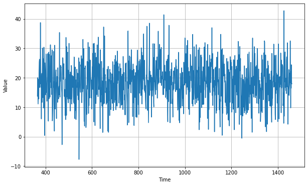
We can then use moving average to forecast this time series which give us these forecasts.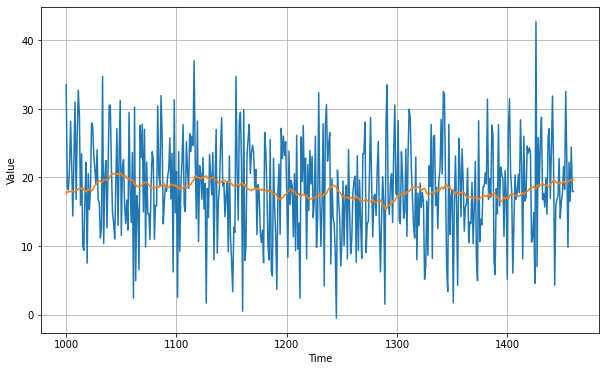
But these are forecast for difference time series not original. To get the final forecasts for the original time series, we just need to add back the value at time T - 365 and we'll get these forecasts
If we measure the mean absolute error on the validation period, we get about 5.8 . So, it's slightly better than naive forecasting but not tremendously better. You may have noticed that our moving average removed a lot of noise but our final forecasts are still pretty noisy.

Where does that noise come from?
Well that's coming from the past values that we added back into our forecasts. So we can improve these forecasts by also removing the past noise using a moving average on that. If we do that, we get much smoother forecasts. The yellow line is the forecast over the blue values of time series data.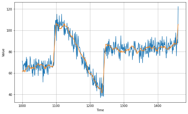
This gives us mean absolute error of 4.5 which is less than our previous forecast. With this approach we're not too far from optimal.

Let's have a look at it's code:

Import Libraries
We'll use tensorflow in the following code.

import tensorflow as tf
import numpy as np
import matplotlib.pyplot as plt
import tensorflow as tf
from tensorflow import keras

Creating Time Series

def plot_series(time, series, format="-", start=0, end=None):
    plt.plot(time[start:end], series[start:end], format)
    plt.xlabel("Time")
    plt.ylabel("Value")
    plt.grid(True)

def trend(time, slope=0):
    return slope * time

def seasonal_pattern(season_time):
    """Just an arbitrary pattern, you can change it if you wish"""
    return np.where(season_time < 0.4,
                    np.cos(season_time * 2 * np.pi),
                    1 / np.exp(3 * season_time))

def seasonality(time, period, amplitude=1, phase=0):
    """Repeats the same pattern at each period"""
    season_time = ((time + phase) % period) / period
    return amplitude * seasonal_pattern(season_time)

def noise(time, noise_level=1, seed=None):
    rnd = np.random.RandomState(seed)
    return rnd.randn(len(time)) * noise_level

time = np.arange(4 * 365 + 1, dtype="float32")
baseline = 10
series = trend(time, 0.1)  
baseline = 10
amplitude = 40
slope = 0.05
noise_level = 5

# Create the series
series = baseline + trend(time, slope) + seasonality(time, period=365, amplitude=amplitude)
# Update with noise
series += noise(time, noise_level, seed=42)

plt.figure(figsize=(10, 6))
plot_series(time, series)
plt.show()

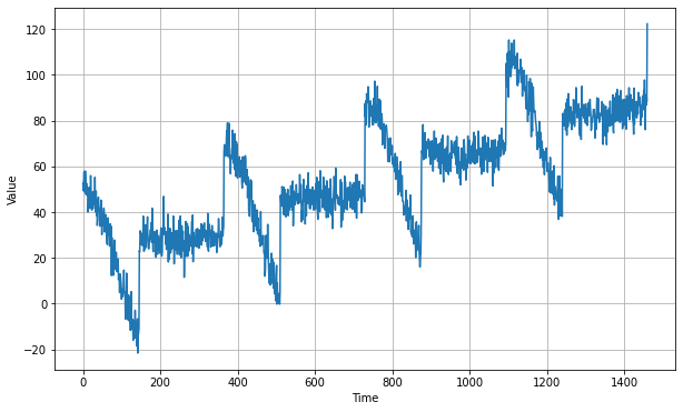
The above code will give us the following series

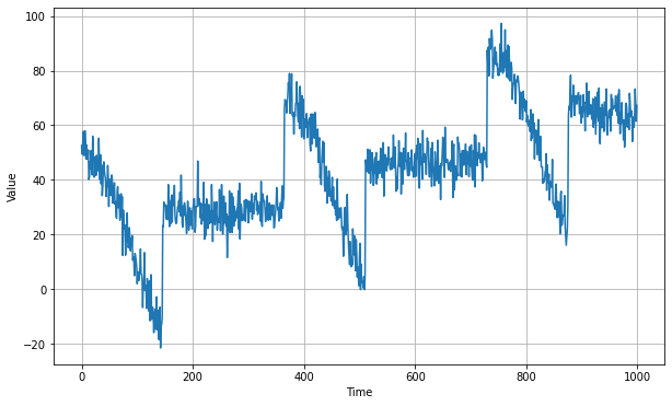
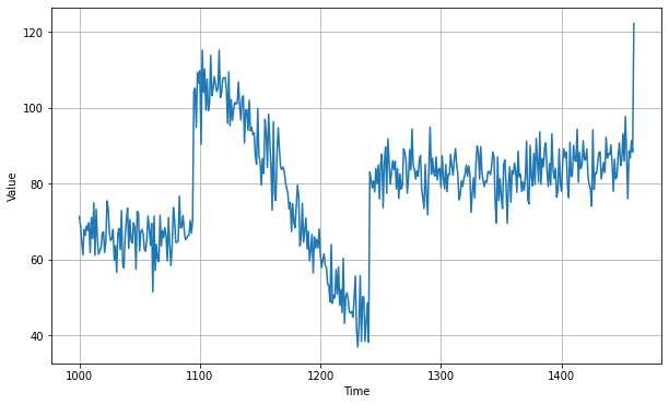
Now that we have the time series, let's split it so we can start forecasting

split_time = 1000
time_train = time[:split_time]
x_train = series[:split_time]
time_valid = time[split_time:]
x_valid = series[split_time:]
plt.figure(figsize=(10, 6))
plot_series(time_train, x_train)
plt.show()

plt.figure(figsize=(10, 6))
plot_series(time_valid, x_valid)
plt.show()

Training period time series data

Validation period time series data

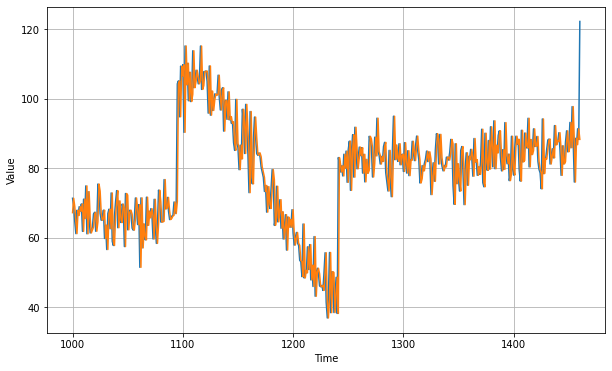
Naive Forecast

naive_forecast = series[split_time - 1:-1]
plt.figure(figsize=(10, 6))
plot_series(time_valid, x_valid)
plot_series(time_valid, naive_forecast)

Naive forecast will give us following forecast plot(yellow line) on the blue values of time series data.

Let's zoom in on the start of the validation period:

plt.figure(figsize=(10, 6))
plot_series(time_valid, x_valid, start=0, end=150)
plot_series(time_valid, naive_forecast, start=1, end=151)

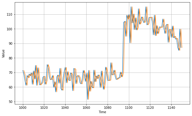
You can see that the naive forecast lags 1 step behind the time series.Now let's compute the mean squared error and the mean absolute error between the forecasts and the predictions in the validation period:

print(keras.metrics.mean_squared_error(x_valid,
naive_forecast).numpy())
print(keras.metrics.mean_absolute_error(x_valid, naive_forecast).numpy())

61.827538
5.9379086

We get 5.93 as our mean absolute error. Let's see if we can do better than this. This is our baseline, now let's try a moving average:

def moving_average_forecast(series, window_size):
  """Forecasts the mean of the last few values.
     If window_size=1, then this is equivalent to naive forecast"""
  forecast = []
  for time in range(len(series) - window_size):
    forecast.append(series[time:time + window_size].mean())
  return np.array(forecast)

moving_avg = moving_average_forecast(series, 30)[split_time - 30:]
plt.figure(figsize=(10, 6))
plot_series(time_valid, x_valid)
plot_series(time_valid, moving_avg)  

This is the forecast line we get after applying moving average method

Let's check it's mean absolute error

print(keras.metrics.mean_squared_error(x_valid, moving_avg).numpy())
print(keras.metrics.mean_absolute_error(x_valid, moving_avg).numpy())

106.674576
7.142419

We got a mean absolute error value of 7.14 which is worse than the naive forecasting value. It happened because it does not anticipate for trend and seasonality. To solve this issue we'll use differencing. Since the seasonality period is 365 days, we will subtract the value at time t – 365 from the value at time t.

diff_series = (series[365:] - series[:-365])
diff_time = time[365:]

diff_moving_avg = moving_average_forecast(diff_series, 50)[split_time - 365 - 50:]

plt.figure(figsize=(10, 6))
plot_series(time_valid, diff_series[split_time - 365:])
plot_series(time_valid, diff_moving_avg)
plt.show()

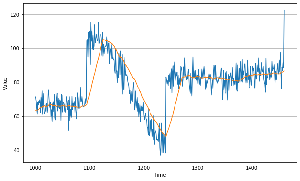
Now let's bring back the trend and seasonality by adding the past values from t – 365:

diff_moving_avg_plus_past = series[split_time - 365:-365] + diff_moving_avg

plt.figure(figsize=(10, 6))
plot_series(time_valid, x_valid)
plot_series(time_valid, diff_moving_avg_plus_past)
plt.show()

print(keras.metrics.mean_squared_error(x_valid, diff_moving_avg_plus_past).numpy())
print(keras.metrics.mean_absolute_error(x_valid, diff_moving_avg_plus_past).numpy())

52.973656
5.8393106

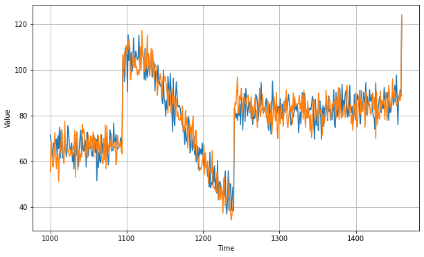
Better than naive forecast, good. However the forecasts look a bit too random, because we're just adding past values, which were noisy. Let's use a moving averaging on past values to remove some of the noise:

diff_moving_avg_plus_smooth_past = moving_average_forecast(series[split_time - 370:-360], 10) + diff_moving_avg

plt.figure(figsize=(10, 6))
plot_series(time_valid, x_valid)
plot_series(time_valid, diff_moving_avg_plus_smooth_past)
plt.show()

print(keras.metrics.mean_squared_error(x_valid, diff_moving_avg_plus_smooth_past).numpy())
print(keras.metrics.mean_absolute_error(x_valid, diff_moving_avg_plus_smooth_past).numpy())

33.45226
4.569442

We can see that we get a much smoother forecasts.This gives us mse of 4.5. With this approach we're not too far from optimal.

In the next part at OpenGenus, we'll do forecasting on time series data using neural network models such as Deep Neural Networks , Recurrent Neural Networks (LSTMs , GRUs etc.) and Convolution neural networks.