In this article, we have explored the 3 different types of Naive Bayes classification algorithm in depth.

Naive Bayes is a classification algorithm based on Bayes' theorem. It is called "naive" because it assumes that the features are independent of each other, which may not be true in real-world scenarios. Despite this simplifying assumption, Naive Bayes is a popular choice for many classification problems due to its simplicity and high accuracy.

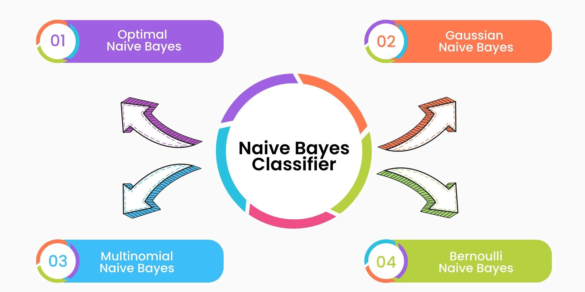
There are three main types of Naive Bayes classifiers:

1. Gaussian Naive Bayes
2. Multinomial Naive Bayes
3. Bernoulli Naive Bayes

1. Gaussian Naive Bayes

Gaussian Naive Bayes is a machine learning algorithm that is commonly used for classification problems. It is a probabilistic algorithm that makes predictions based on the probability of each possible outcome. In this algorithm, the term 'Naive' is used because it makes a strong assumption that all features are independent of each other, given the class label. This means that the algorithm considers each feature individually and assumes that they contribute equally to the probability of the class.

The algorithm works by first estimating the probability distribution of each feature, given the class label. It does this by calculating the mean and standard deviation of each feature for each class label. The mean represents the average value of the feature for that class, while the standard deviation represents the variability of the feature for that class.

Once the probability distributions have been estimated, the algorithm can make predictions on new data. Given a set of features for a new data point, the algorithm calculates the probability of each possible class label, given those features. It does this by using Bayes' theorem, which states that:

P(y|x) = (P(x|y) * P(y)) / P(x)

where P(y|x) is the probability of the class label y given the features x, P(x|y) is the probability of the features x given the class label y, P(y) is the prior probability of the class label y, and P(x) is the probability of the features x.

In Gaussian Naive Bayes, the assumption is made that the probability distribution of each feature given the class label is Gaussian (i.e., normally distributed). Therefore, the probability of the features x given the class label y can be calculated using the Gaussian probability density function:

P(x|y) = (1 / (sqrt(2 * pi) * sigma)) * exp(-(x - mu)^2 / (2 * sigma^2))

where mu is the mean of the feature for the class label y, sigma is the standard deviation of the feature for the class label y, and pi is the mathematical constant.

To make a prediction on a new data point, the algorithm calculates the probability of each possible class label using the above formula, and then selects the class label with the highest probability.

The algorithm is called 'Naive' because it assumes that all features are independent of each other, given the class label. In reality, this assumption may not hold true for all datasets. However, even with this assumption, Gaussian Naive Bayes can be a powerful and efficient

Advantages and Disadvantages of Gaussian Naive Bayes

Advantages:

1. GNB is a simple and easy-to-understand algorithm that is relatively easy to implement.
2. It is computationally efficient and can handle large datasets with high dimensionality.
3. GNB works well with small and medium-sized datasets and is especially effective when the number of features is relatively small compared to the number of observations.
4. GNB performs well even in cases where the independence assumption of features does not hold exactly.
5. GNB can handle missing data values by ignoring them during model building.

Disadvantages:

1. GNB assumes that the features are independent of each other, which may not be true in some cases. This can lead to inaccurate results.
2. GNB cannot handle correlated features or interactions between features. In such cases, a more sophisticated algorithm may be required.
3. GNB is not suitable for tasks that require probabilities to be calibrated. The algorithm often produces probabilities that are not well-calibrated, which can make it unsuitable for some applications.
4. GNB can be sensitive to outliers in the data. Outliers can affect the mean and variance of the feature values, which can lead to inaccurate results.
5. GNB is not suitable for handling text or image data, where the feature space can be very large and the features are not necessarily independent.

Overall, GNB is a simple and efficient algorithm that can work well in many classification problems, especially with small to medium-sized datasets. However, it may not be the best choice for problems with complex or highly correlated features, or those that require well-calibrated probabilities.

2. Multinomial Naive Bayes

Multinomial Naive Bayes is a classification algorithm based on Bayes' theorem that is used for categorizing documents or text into multiple classes. It is a popular algorithm used in Natural Language Processing (NLP) applications such as spam detection, sentiment analysis, and text classification.

How Multinomial Naive Bayes Works
Multinomial Naive Bayes is a probabilistic algorithm that assumes the independence of the features (words) in the input data. It uses Bayes' theorem to compute the probability of each class given the input features.

Bayes' theorem states that:
P(y|x) = (P(x|y) * P(y)) / P(x)

where:

• P(y|x) is the probability of class y given the input x.
• P(x|y) is the probability of input x given the class y.
• P(y) is the prior probability of class y.
• P(x) is the probability of input x.

In text classification, the input x is a document or text, and the classes y are the different categories or labels that we want to classify the text into. The goal is to find the class y that has the highest probability given the input x.

The algorithm uses the bag-of-words model to represent the input text as a vector of word frequencies. Each word in the input text is treated as a feature, and its frequency in the document is the value of that feature.

To compute the probability of each class given the input features, the algorithm first calculates the prior probability of each class. This is the probability of each class based on the frequency of the class labels in the training data.

Next, the algorithm calculates the likelihood of each feature given each class. This is the probability of each word occurring in the training data for each class.

Finally, the algorithm combines the prior probability and likelihood to compute the probability of each class given the input features using Bayes' theorem.

Advantages and Disadvantages of Multinomial Naive Bayes

Advantages:
Simple and easy to implement.
Works well with high-dimensional sparse data, which is common in text classification.
Can handle a large number of classes.

Disadvantages:
Assumes independence of features, which may not be true in practice.
Requires a large amount of training data to estimate the parameters accurately.
Can be sensitive to irrelevant features, leading to overfitting.

Multinomial Naive Bayes is a powerful and widely used algorithm for text classification tasks. It works well with high-dimensional sparse data and can handle a large number of classes. However, it has some limitations and assumptions that need to be considered when applying the algorithm in practice.

3. Bernoulli Naive Bayes

Bernoulli Naive Bayes is a classification algorithm that is based on the Bayes' theorem. It is a probabilistic model that predicts the probability of a sample belonging to a particular class. In the case of Bernoulli Naive Bayes, it is used for binary classification problems, where the target variable can take only two values, usually 0 or 1.

The algorithm assumes that each feature is independent of all other features and follows a Bernoulli distribution. This means that each feature can only take two possible values, 0 or 1, and that the probability of each feature being 1 is the same for all samples.

The algorithm works by first calculating the prior probability of each class, which is the probability of a sample belonging to that class without considering any features. This is calculated as the number of samples in that class divided by the total number of samples.

Next, for each feature, the algorithm calculates the likelihood of that feature given each class. This is done by calculating the probability of that feature being 1 in the samples belonging to that class.

Finally, the algorithm calculates the posterior probability of each class given the features of the sample using Bayes' theorem. The posterior probability is the probability of a sample belonging to a particular class given its features. The class with the highest posterior probability is predicted as the class for the sample.

The mathematical formula for Bernoulli Naive Bayes is as follows:

P(y|x) = P(y) * ∏ P(xi|y)

Where:

• P(y|x) is the posterior probability of class y given the features x
• P(y) is the prior probability of class y
• P(xi|y) is the likelihood of feature i given class y
• ∏ is the product symbol

To avoid the problem of zero probabilities, which can occur if a feature is absent from the training data for a particular class, a smoothing technique called Laplace smoothing is used. This involves adding a small constant value to the numerator and denominator of each likelihood calculation.

Bernoulli Naive Bayes is a simple and efficient algorithm that works well for text classification problems and other problems where the features are binary. However, it may not perform as well as other algorithms when the features are not independent or when the data has a large number of features.

Advantages and Disadvantages of Bernoulli Naive Bayes

Advantages:

1. Simplicity: Bernoulli Naive Bayes is a simple algorithm that is easy to understand and implement. It is also computationally efficient, making it a good choice for large datasets.
2. Works well with binary data: Bernoulli Naive Bayes works well with binary data, which is data that only takes on two possible values (such as 0 and 1). It is particularly useful for text classification problems where the presence or absence of certain words is used as features.
3. Requires less training data: Bernoulli Naive Bayes requires less training data compared to other classification algorithms, making it a good choice when the dataset is small.
4. Robust to irrelevant features: Bernoulli Naive Bayes is robust to irrelevant features, meaning that it can still produce accurate results even when some of the features are not relevant to the classification problem.

Disadvantages:

1. Assumes independence between features: Bernoulli Naive Bayes assumes that the features are independent of each other, which is not always the case in real-world datasets. This can lead to inaccurate results.
2. Cannot handle continuous data: Bernoulli Naive Bayes cannot handle continuous data, which is data that takes on a continuous range of values. This can be a problem when dealing with datasets that contain continuous features.
3. Limited expressive power: Bernoulli Naive Bayes has limited expressive power compared to other classification algorithms. This means that it may not be able to capture complex relationships between the features and the target variable.
4. Requires feature selection: Bernoulli Naive Bayes requires feature selection, which means that only relevant features should be used as input. This can be a time-consuming process and may require domain knowledge.

With this article at OpenGenus, you must have the complete idea of different Naive Bayes algorithms.